In December, Statistics Canada refreshed their National Address Register (NAR). This is a database containing 15,819,286 civic addresses for Canada.
In this post, I'll download these addresses and use them to create centroids for Canada's major settlements.
My Workstation
I'm using a 5.7 GHz AMD Ryzen 9 9950X CPU. It has 16 cores and 32 threads and 1.2 MB of L1, 16 MB of L2 and 64 MB of L3 cache. It has a liquid cooler attached and is housed in a spacious, full-sized Cooler Master HAF 700 computer case.
The system has 96 GB of DDR5 RAM clocked at 4,800 MT/s and a 5th-generation, Crucial T700 4 TB NVMe M.2 SSD which can read at speeds up to 12,400 MB/s. There is a heatsink on the SSD to help keep its temperature down. This is my system's C drive.
The system is powered by a 1,200-watt, fully modular Corsair Power Supply and is sat on an ASRock X870E Nova 90 Motherboard.
I'm running Ubuntu 24 LTS via Microsoft's Ubuntu for Windows on Windows 11 Pro. In case you're wondering why I don't run a Linux-based desktop as my primary work environment, I'm still using an Nvidia GTX 1080 GPU which has better driver support on Windows and I use ArcGIS Pro from time to time which only supports Windows natively.
Installing Prerequisites
I'll use Python 3.12.3 and jq to help analyse the data in this post.
$ sudo add-apt-repository ppa:deadsnakes/ppa
$ sudo apt update
$ sudo apt install \
    jq \
    python3-pip \
    python3.12-venv
I'll set up a Python Virtual Environment and install the latest AWS CLI release.
$ python3 -m venv ~/.statscan
$ source ~/.statscan/bin/activate
$ python3 -m pip install \
    awscli
I'll use DuckDB, along with its H3, JSON, Lindel, Parquet and Spatial extensions, in this post.
$ cd ~
$ wget -c https://github.com/duckdb/duckdb/releases/download/v1.1.3/duckdb_cli-linux-amd64.zip
$ unzip -j duckdb_cli-linux-amd64.zip
$ chmod +x duckdb
$ ~/duckdb
INSTALL h3 FROM community;
INSTALL lindel FROM community;
INSTALL json;
INSTALL parquet;
INSTALL spatial;
I'll set up DuckDB to load every installed extension each time it launches.
$ vi ~/.duckdbrc
.timer on
.width 180
LOAD h3;
LOAD lindel;
LOAD json;
LOAD parquet;
LOAD spatial;
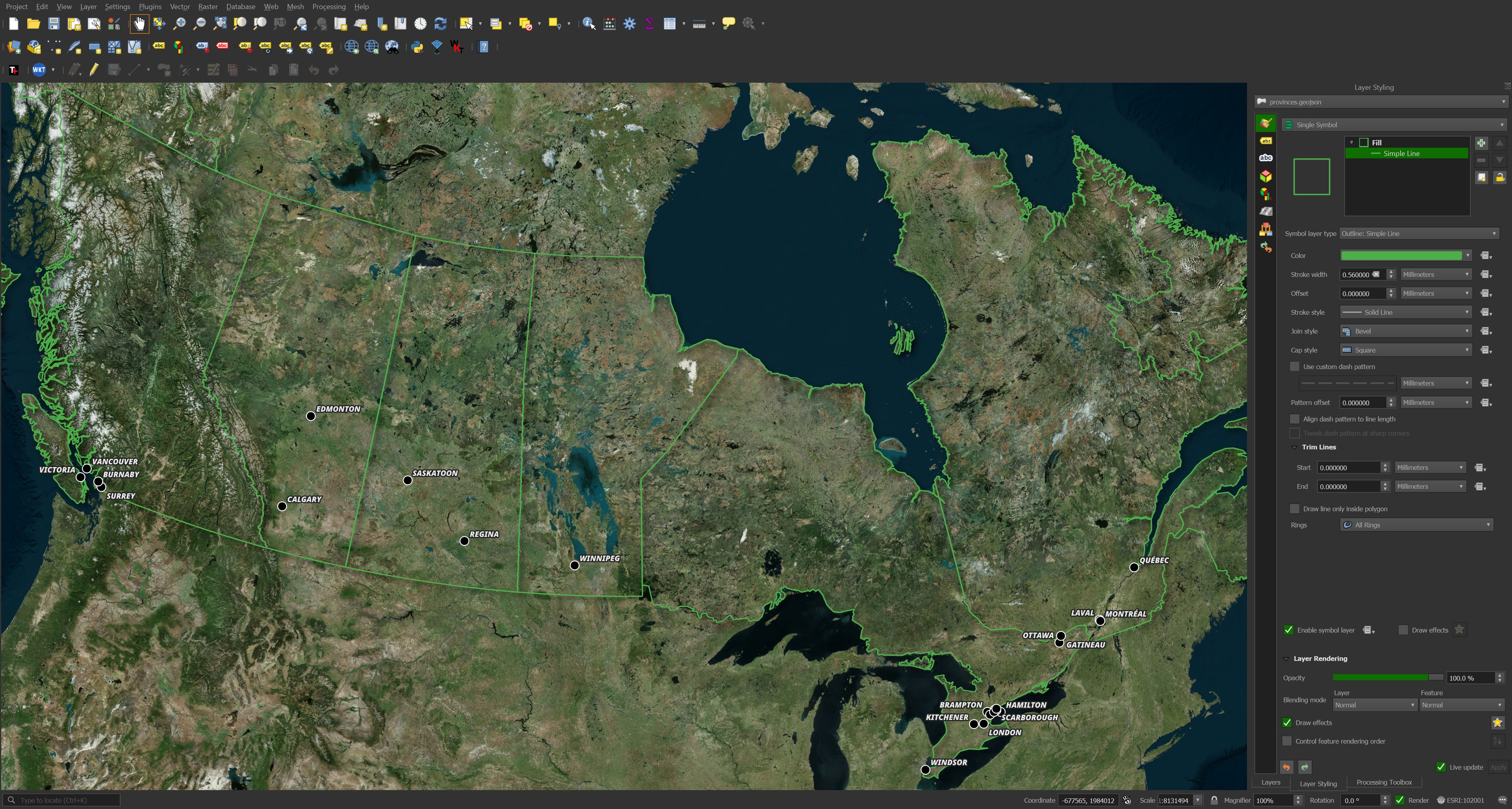
The maps in this post were rendered with QGIS version 3.42. QGIS is a desktop application that runs on Windows, macOS and Linux. The application has grown in popularity in recent years and has ~15M application launches from users all around the world each month.
I used QGIS' Tile+ plugin to add geospatial context with Bing's Virtual Earth Basemap as well as OpenStreetMap's (OSM) and CARTO's to the maps.
I found a GeoJSON file on GitHub that outlines Canada's Provinces pretty well.
Statistics Canada's National Address Register
I'll download Statistics Canada's 1.7 GB ZIP file.
$ wget https://www150.statcan.gc.ca/n1/pub/46-26-0002/2022001/202412.zip
$ unzip 202412.zip
The above ZIP file contains 3.2 GB of address data across 27 CSV files as well as 1.7 GB of location data across 22 CSV files. For this exercise, I'll be convert the address data into Parquet.
Below I'll reproject the geometry to EPSG:4326 as well as calculate a bounding box around each record. This will make it easier to filter out records of interest without needing to read the entire file.
I'll sort the records spatially and use the strongest compression ZStandard offers.
$ ~/duckdb
COPY (
    SELECT   * EXCLUDE(BG_X, BG_Y),
             ST_ASWKB(
                ST_FLIPCOORDINATES(
                    ST_TRANSFORM(ST_POINT(BG_X, BG_Y),
                                 'EPSG:3347',
                                 'EPSG:4326'))) geom,
             {'xmin': ST_XMIN(ST_EXTENT(geom)),
              'ymin': ST_YMIN(ST_EXTENT(geom)),
              'xmax': ST_XMAX(ST_EXTENT(geom)),
              'ymax': ST_YMAX(ST_EXTENT(geom))} AS bbox
    FROM     READ_CSV('Addresses/*.csv')
    WHERE    BG_X IS NOT NULL
    AND      BG_Y IS NOT NULL
    ORDER BY HILBERT_ENCODE([ST_Y(
                                ST_CENTROID(
                                    ST_TRANSFORM(ST_POINT(BG_X, BG_Y),
                                                 'EPSG:3347',
                                                 'EPSG:4326'))),
                             ST_X(
                                ST_CENTROID(
                                    ST_TRANSFORM(ST_POINT(BG_X, BG_Y),
                                                 'EPSG:3347',
                                                 'EPSG:4326')))]::double[2])
) TO 'addresses.pq' (
    FORMAT            'PARQUET',
    CODEC             'ZSTD',
    COMPRESSION_LEVEL 22,
    ROW_GROUP_SIZE    15000);
The resulting Parquet file is 852 MB. Below is an example record.
$ echo "FROM  READ_PARQUET('addresses.pq')
        WHERE LOC_GUID = '13e7e958-f46d-4f88-aede-14fd9455fbe3'
        LIMIT 1" \
    | ~/duckdb -json \
    | jq -S .
[
  {
    "ADDR_GUID": "77bf56c5-3b0a-4e6d-9b45-95f6546d59d3",
    "APT_NO_LABEL": null,
    "BG_DLS_LSD": null,
    "BG_DLS_MRD": "W5",
    "BG_DLS_QTR": "SE",
    "BG_DLS_RNG": "1",
    "BG_DLS_SCTN": "15",
    "BG_DLS_TWNSHP": "24",
    "BU_N_CIVIC_ADD": null,
    "BU_USE": 3,
    "CIVIC_NO": 555,
    "CIVIC_NO_SUFFIX": null,
    "CSD_ENG_NAME": "Calgary",
    "CSD_FRE_NAME": "Calgary",
    "CSD_TYPE_ENG_CODE": "CY",
    "CSD_TYPE_FRE_CODE": "CY",
    "LOC_GUID": "13e7e958-f46d-4f88-aede-14fd9455fbe3",
    "MAIL_MUN_NAME": "CALGARY",
    "MAIL_POSTAL_CODE": "T2G2W1",
    "MAIL_PROV_ABVN": "AB",
    "MAIL_STREET_DIR": "SE",
    "MAIL_STREET_NAME": "SADDLEDOME",
    "MAIL_STREET_TYPE": "RISE",
    "OFFICIAL_STREET_DIR": "SE",
    "OFFICIAL_STREET_NAME": "Saddledome",
    "OFFICIAL_STREET_TYPE": "RISE",
    "PROV_CODE": 48,
    "bbox": "{'xmin': -114.05352113882974, 'ymin': 51.03819428139459, 'xmax': -114.05352113882974, 'ymax': 51.03819428139459}",
    "geom": "POINT (-114.05352113882974 51.03819428139459)"
  }
]
Only Read What You Need
The bounding box field contains four floating point columns. These will have statistics of their minimum and maximum values for every 15K rows. Certain queries can rely on these statistics alone to return results.
Below I'll upload the 852 MB Parquet file to Amazon's S3 region in Calgary and get its signed URL.
$ aws s3 cp \
    addresses.pq \
    s3://<bucket>/addresses.pq

$ aws s3 presign  \
    --expires-in 3600 \
    --region ca-west-1 \
    --endpoint-url https://s3.ca-west-1.amazonaws.com \
    s3://<bucket>/addresses.pq
I'll then count how many addresses exist within a given bounding box.
$ ~/duckdb
EXPLAIN ANALYZE
    SELECT COUNT(*)
    FROM   READ_PARQUET('https://s3.ca-west-1.amazonaws.com/...')
    WHERE  bbox.xmin BETWEEN -120 AND -119
    AND    bbox.ymin BETWEEN   53 AND   54;
The resulting answer only needed to read 3 MB of data, not the entire 852 MB file. It was able to read this data across five separate HTTPS requests and only took 1.46 seconds to run.
┌─────────────────────────────────────┐
│┌───────────────────────────────────┐│
││         HTTPFS HTTP Stats         ││
││                                   ││
││            in: 3.0 MiB            ││
││            out: 0 bytes           ││
││              #HEAD: 1             ││
││              #GET: 5              ││
││              #PUT: 0              ││
││              #POST: 0             ││
│└───────────────────────────────────┘│
└─────────────────────────────────────┘
┌────────────────────────────────────────────────┐
│┌──────────────────────────────────────────────┐│
││               Total Time: 1.46s              ││
│└──────────────────────────────────────────────┘│
└────────────────────────────────────────────────┘
┌───────────────────────────┐
│           QUERY           │
└─────────────┬─────────────┘
┌─────────────┴─────────────┐
│      EXPLAIN_ANALYZE      │
│    ────────────────────   │
│           0 Rows          │
│          (0.00s)          │
└─────────────┬─────────────┘
┌─────────────┴─────────────┐
│    UNGROUPED_AGGREGATE    │
│    ────────────────────   │
│        Aggregates:        │
│        count_star()       │
│                           │
│           1 Rows          │
│          (0.00s)          │
└─────────────┬─────────────┘
┌─────────────┴─────────────┐
│         TABLE_SCAN        │
│    ────────────────────   │
│         Function:         │
│        READ_PARQUET       │
│                           │
│          Filters:         │
│ bbox.xmin>=-120.0 AND bbox│
│   .xmin<=-119.0 AND bbox  │
│ .xmin IS NOT NULL AND bbox│
│ .ymin>=53.0 AND bbox.ymin<│
│ =54.0 AND bbox.ymin IS NOT│
│            NULL           │
│                           │
│          251 Rows         │
│          (4.56s)          │
└───────────────────────────┘
Canada's Settlements
The above dataset contains 7,623 unique province-municipality pairs. I'll calculate a bounding box around each of them and export the result to a GeoPackage (GPKG) file.
$ ~/duckdb
COPY (
    SELECT   MAIL_PROV_ABVN,
             MAIL_MUN_NAME,
             ST_CENTROID({
                'min_x': MIN(ST_X(geom)),
                'min_y': MIN(ST_Y(geom)),
                'max_x': MAX(ST_X(geom)),
                'max_y': MAX(ST_Y(geom))}::BOX_2D::GEOMETRY) AS geom,
             COUNT(*) num_addresses
    FROM     READ_PARQUET('addresses.pq')
    WHERE    MAIL_PROV_ABVN IS NOT NULL
    AND      MAIL_MUN_NAME  IS NOT NULL
    GROUP BY 1, 2
) TO 'nar.centroids.gpkg'
    WITH (FORMAT GDAL,
          DRIVER 'GPKG',
          LAYER_CREATION_OPTIONS 'WRITE_BBOX=YES');
I'll then filter on settlements with at least 100K addresses.
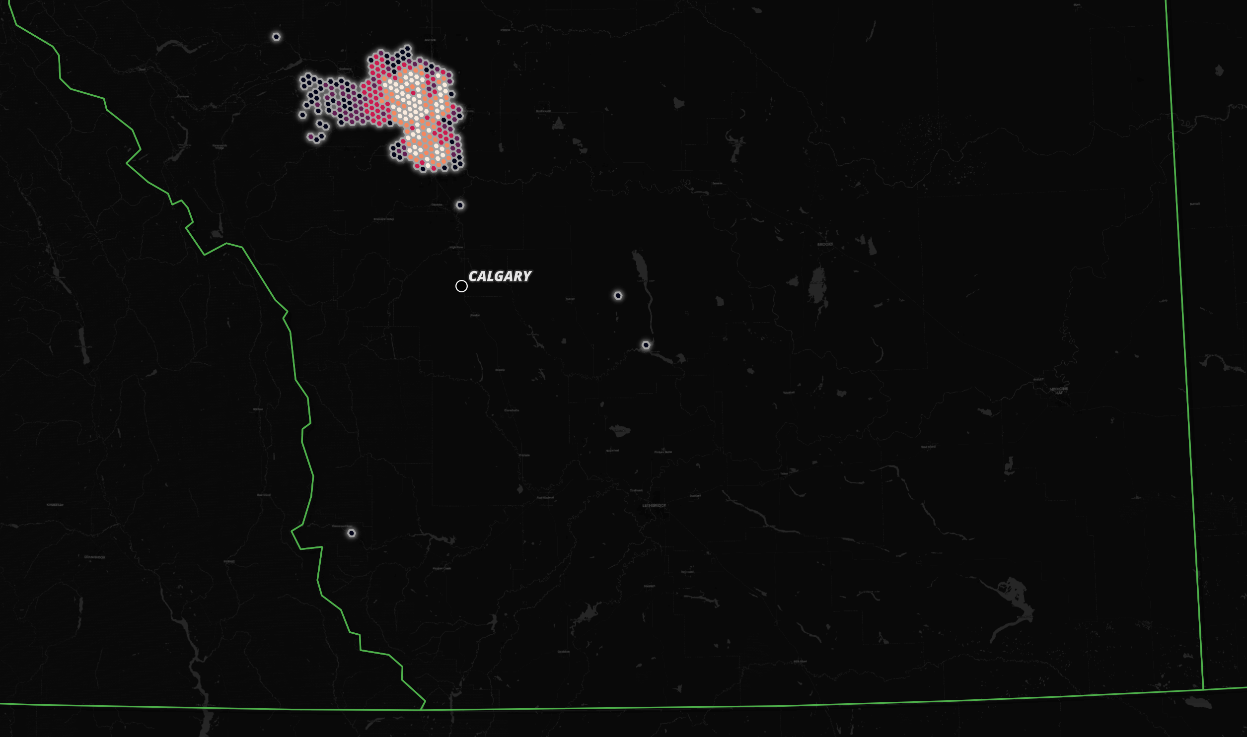
The above looks pretty good but when I zoom into any one city, the centroid location is very far away from the downtown area. It turns out addresses very far away from the city centre might still be classified as being in that city.
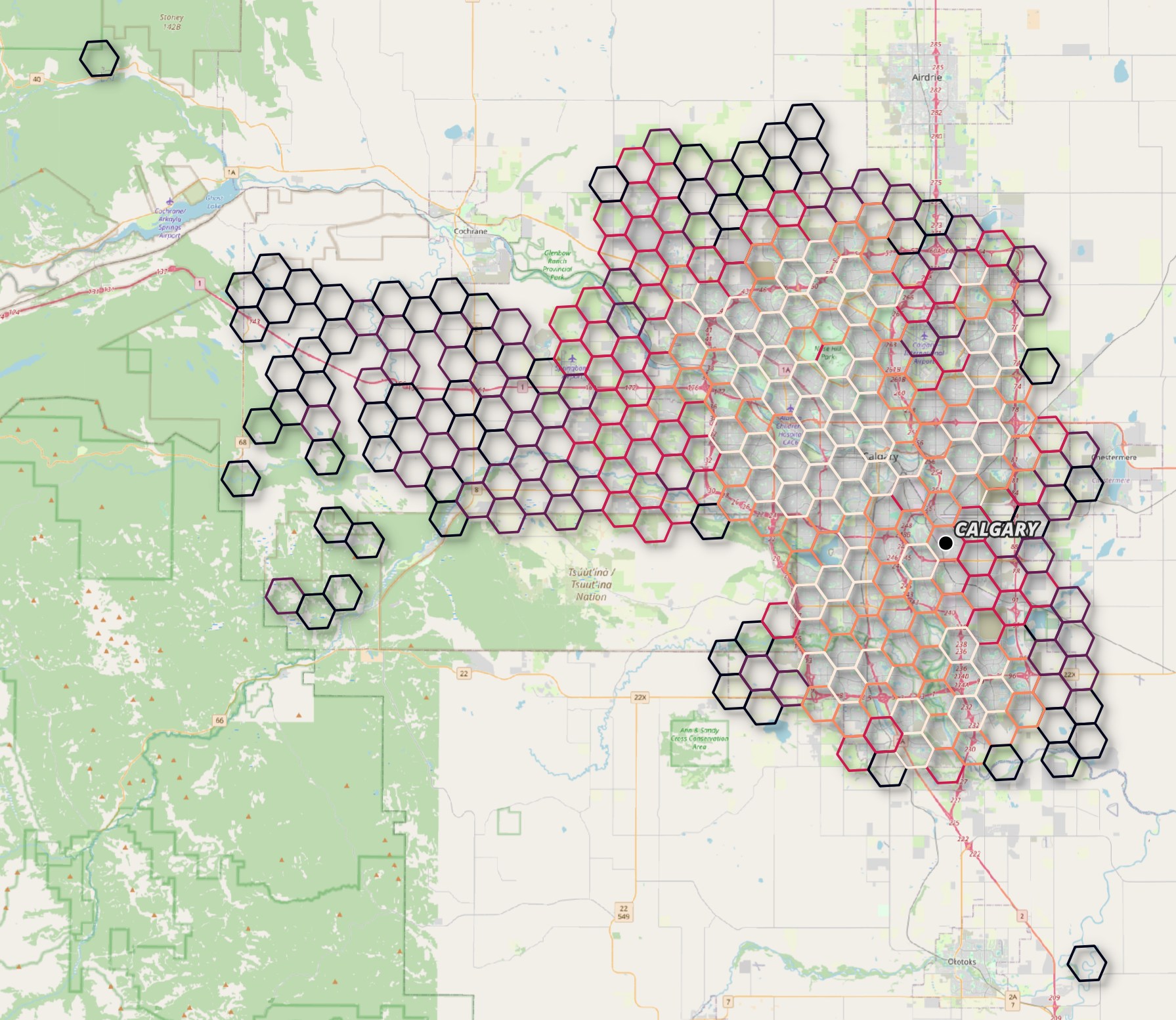
A Hexagon Heatmap
I'll cluster addresses for each provide-municipality pair by their H3 zoom level 5 hexagon and pick the hexagon for each provide-municipality pair with the largest number of addresses.
$ ~/duckdb
CREATE OR REPLACE TABLE centroids AS
    WITH b AS (
        WITH a AS (
            SELECT   h3_cell_to_boundary_wkt(
                          h3_latlng_to_cell(ST_Y(geom),
                                            ST_X(geom),
                                            5))::GEOMETRY geom,
                     MAIL_PROV_ABVN,
                     MAIL_MUN_NAME,
                     COUNT(*) num_addresses
            FROM     READ_PARQUET('addresses.pq')
            GROUP BY 1, 2, 3
        )
        SELECT *,
               ROW_NUMBER() OVER (PARTITION BY MAIL_PROV_ABVN,
                                               MAIL_MUN_NAME
                                  ORDER BY     num_addresses DESC) AS rn
        FROM   a
    )
    FROM     b
    WHERE    rn = 1
    ORDER BY num_addresses DESC;
I'll export the top hexagon for each provide-municipality pair to a GPKG file.
COPY (
    SELECT ST_CENTROID(geom),
           MAIL_PROV_ABVN,
           MAIL_MUN_NAME,
           num_addresses
    FROM   centroids
    WHERE  MAIL_PROV_ABVN IS NOT NULL
    AND    MAIL_MUN_NAME  IS NOT NULL
) TO 'nar.centroids.gpkg'
    WITH (FORMAT GDAL,
          DRIVER 'GPKG',
          LAYER_CREATION_OPTIONS 'WRITE_BBOX=YES');
Now when I filter on settlements with at least 100K addresses, each centroid is much closer to their respective city centre. Below Calgary's centroid is outside of the downtown area but not by much. This is much better than the previous centroid which was a long drive south of Calgary's city limits.
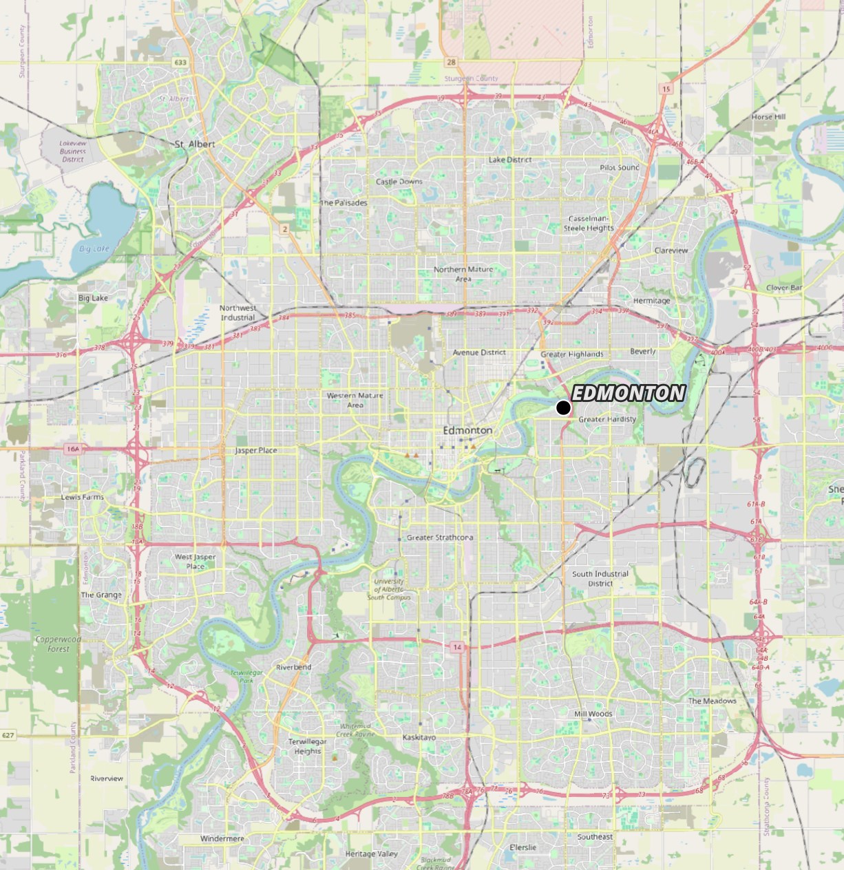
Below is Edmonton's centroid.
These are the centroids for Vancouver and Surrey.
