Capella Space is an 8-year-old manufacturer and operator of a Synthetic Aperture Radar (SAR) satellite fleet. These satellites can see through clouds, smoke and rain and can capture images day or night at resolutions as fine as 32cm. The company has raised $250M to date and has 200 employees working towards building an operational fleet of 36 satellites.
The size of the fleet is important as with 12 orbital planes, 36 satellites could revisit any location on Earth every hour.
SpaceX and Rocket Lab are Capella's launch partners and as of this writing, five of Capella's satellites are in orbit and are operational. Below are Capella's launch dates for its fleet both past and planned for this year.
Name        | Generation-# | Launched  | Launch Rocket
------------|--------------|-----------|--------------
Capella-1   | Denali       | 03 Dec 18 | Falcon 9 B5
Capella-2   | Sequoia      | 31 Aug 20 | Electron
Capella-3   | Whitney-1    | 24 Jan 21 | Falcon 9 B5
Capella-4   | Whitney-2    | 24 Jan 21 | Falcon 9 B5
Capella-5   | Whitney-3    | 30 Jun 21 | Falcon 9 B5
Capella-6   | Whitney-4    | 15 May 21 | Falcon 9 B5
Capella-7   | Whitney-5    | 13 Jan 22 | Falcon 9 B5
Capella-8   | Whitney-6    | 13 Jan 22 | Falcon 9 B5
Capella-9   | Whitney-7    | 16 Mar 23 | Electron
Capella-10  | Whitney-8    | 16 Mar 23 | Electron
Capella-11  | Acadia-1     | 23 Aug 23 | Electron
Capella-12  | Acadia-2     | 19 Sep 23 | Electron
Capella-13  | Acadia-3     |      2024 | Electron
Capella-14  | Acadia-4     | 07 Apr 24 | Falcon 9
Capella-15  | Acadia-5     |      2024 | Falcon 9
Capella-16  | Acadia-6     |      2024 | Falcon 9
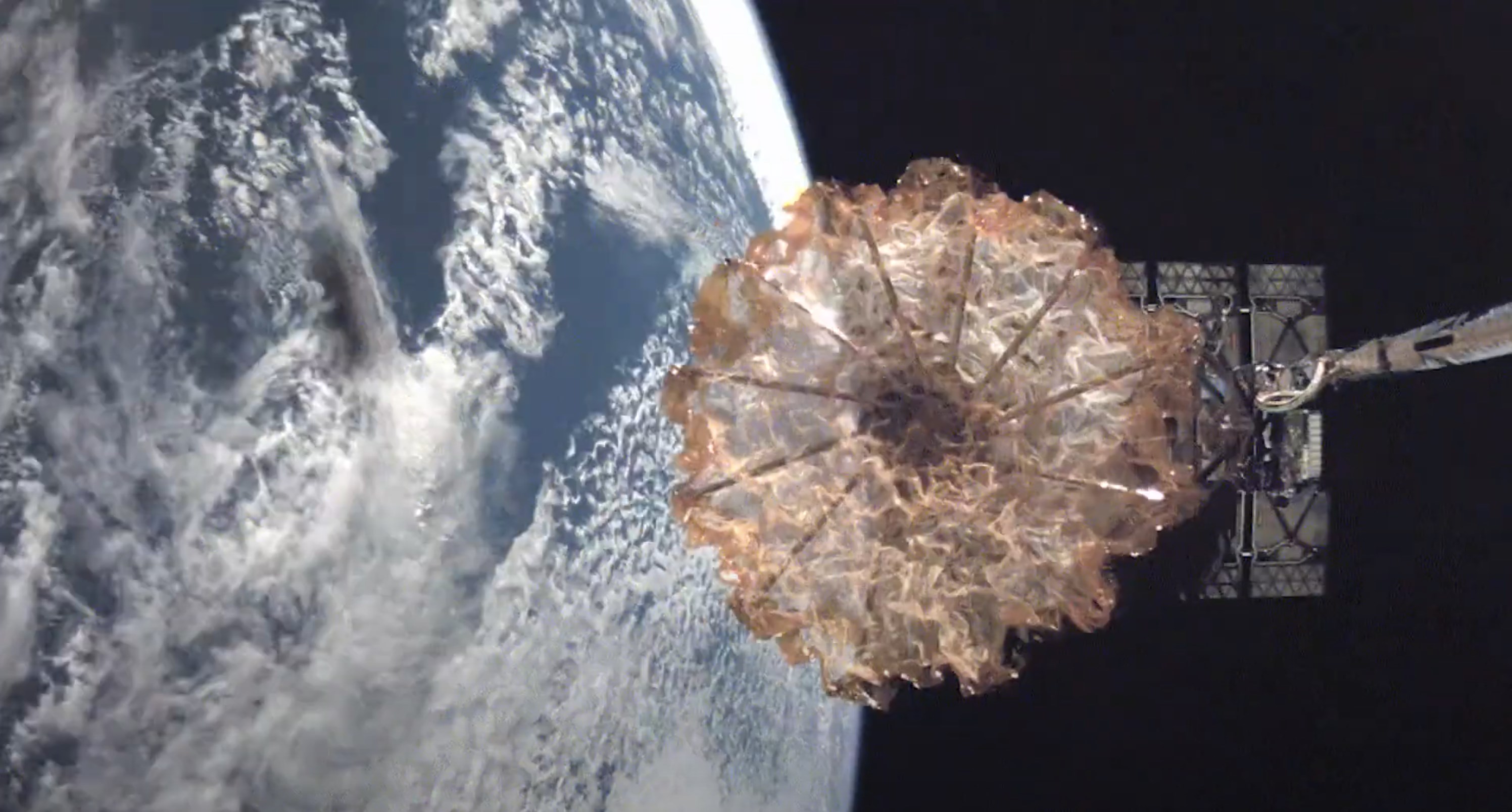
Below is one of Capella's satellites being deployed in 2021.
Capella's imagery typically has a footprint of 5 x 5 KM. Below is an example image taken in India.
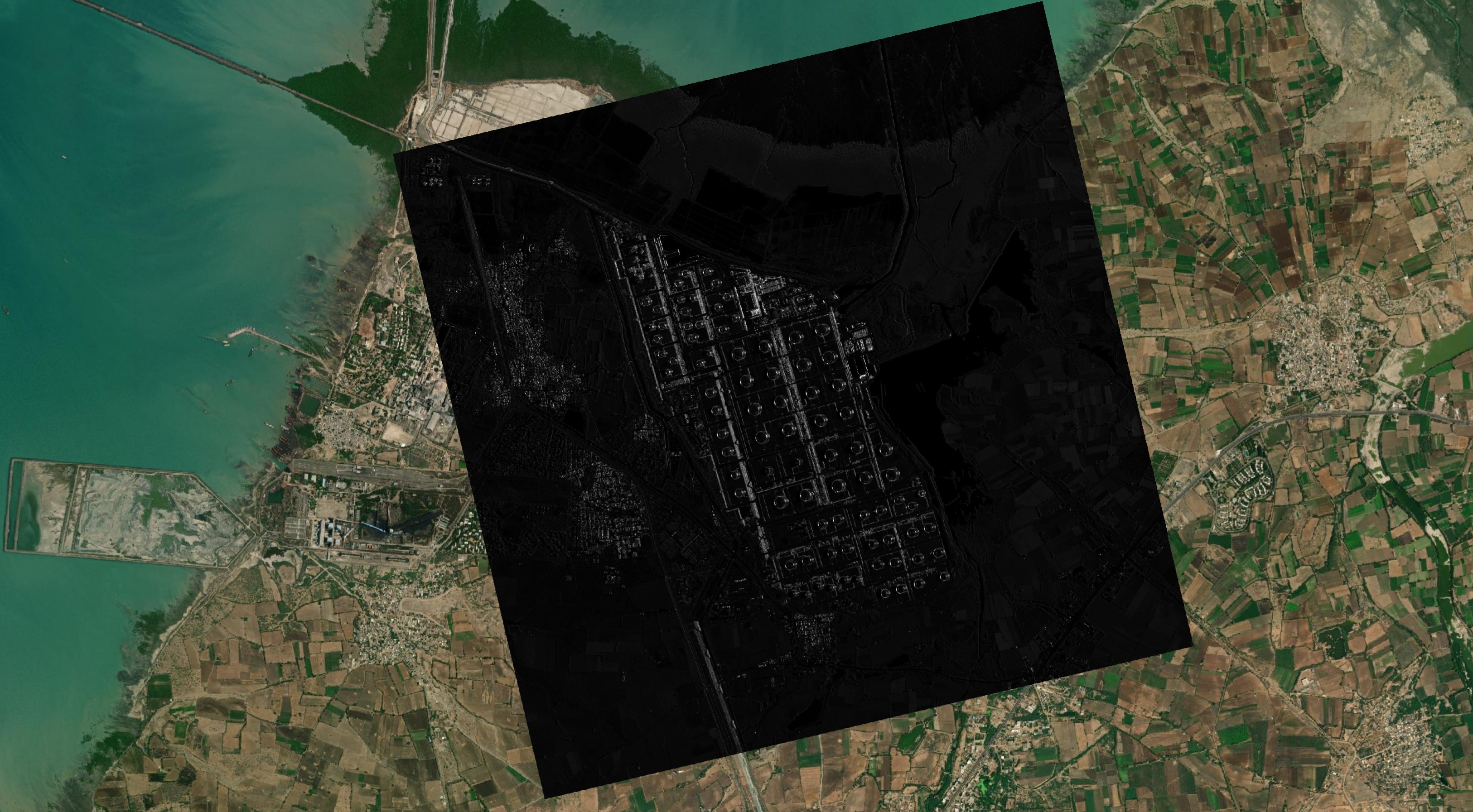
The images are very detailed and man-made objects stand out well. Below I've zoomed into the above image and tinted it pink in QGIS.

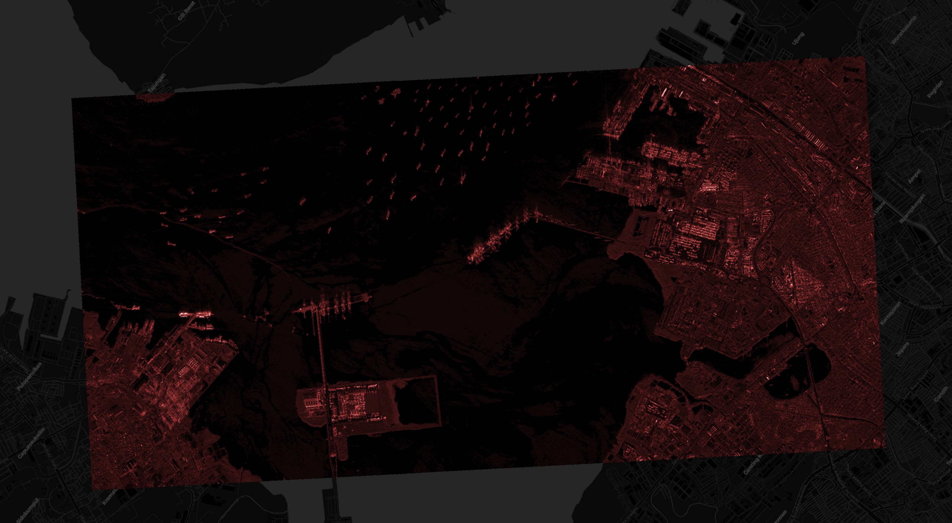
Below are a large number of boats in Surabaya, Indonesia.
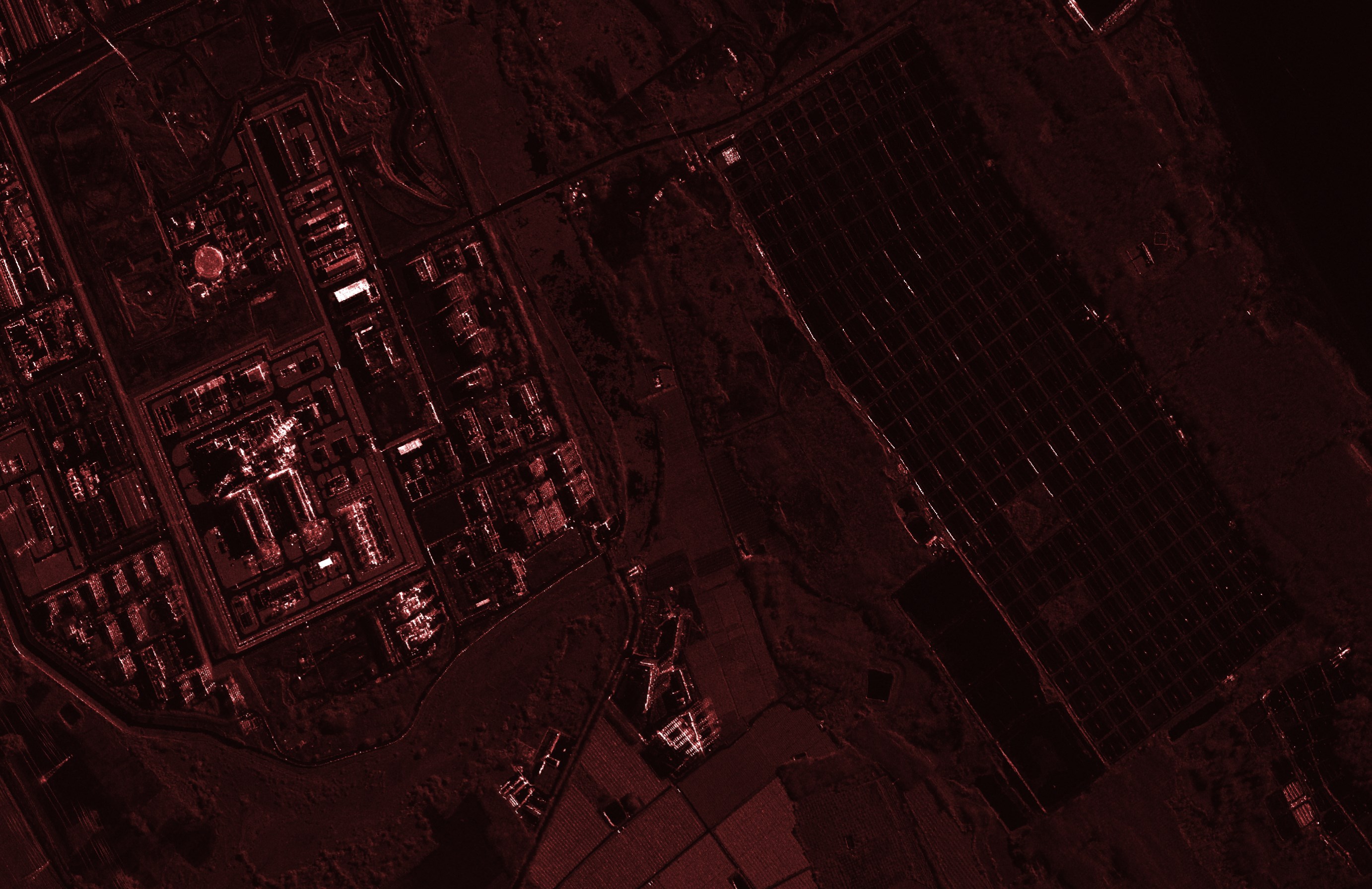
Solar Farms can be seen regardless if it is a cloudy day or not.
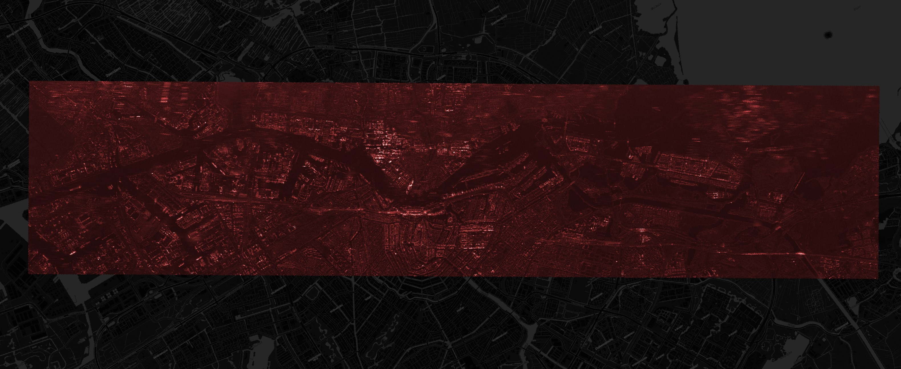
There are also long images where one dimension is 20-40 KM long. The image below is of Amsterdam and covers an area of 5 x 20 KM.
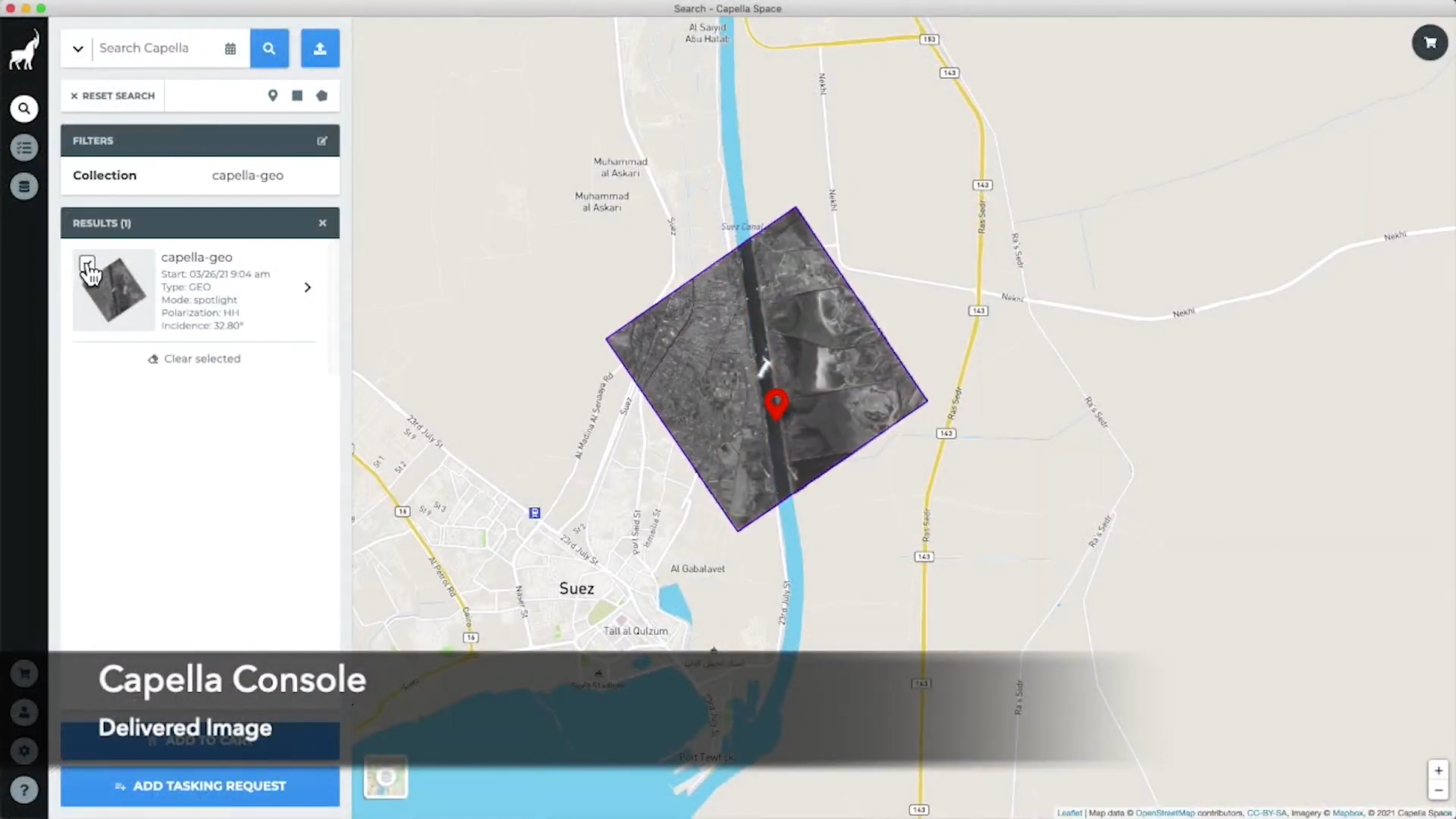
Below is a screenshot of their Tasking UI as an order is being placed for an image of the Ever Given ship that got stuck in the Suez Canal in 2021.
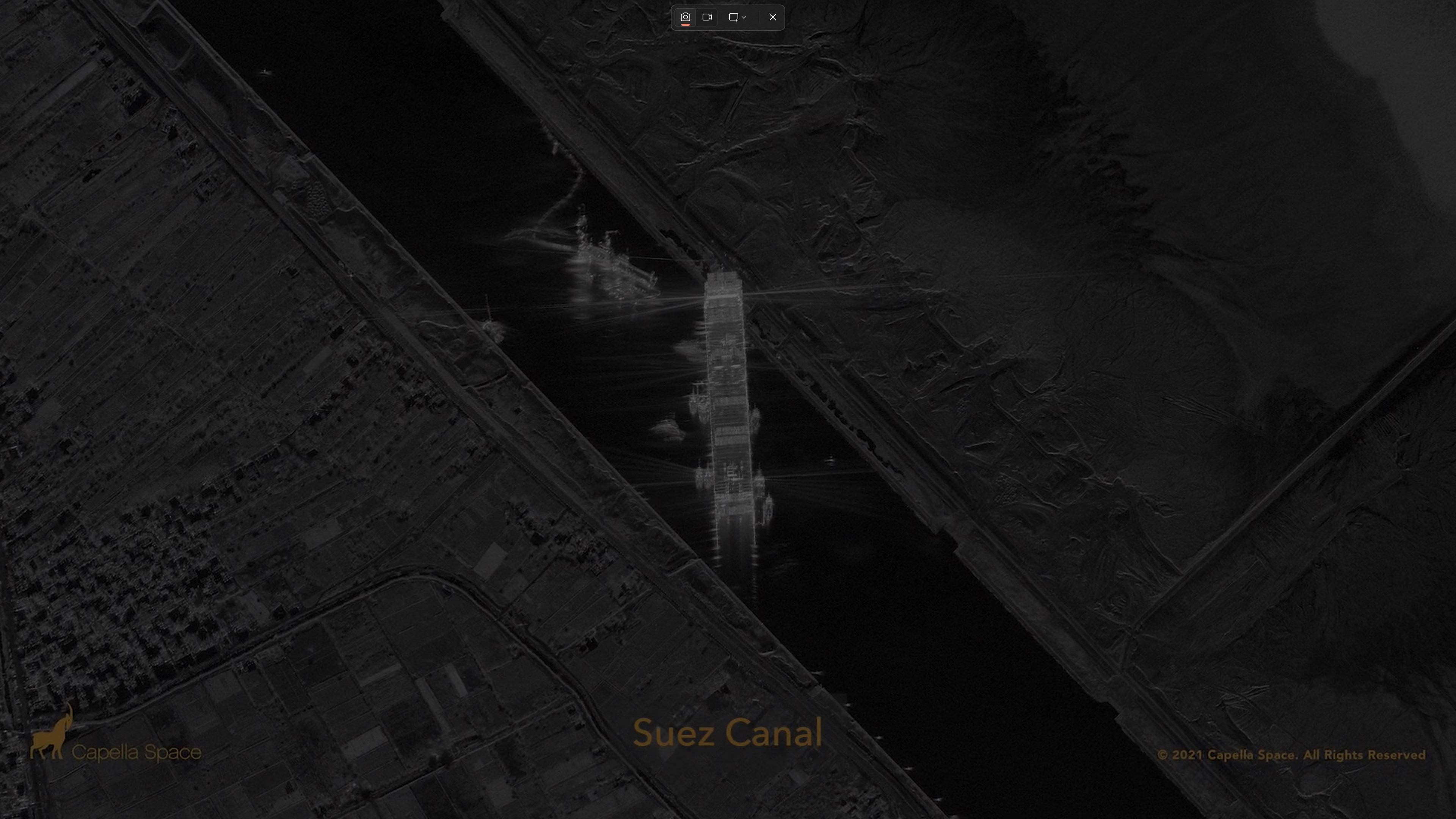
This is a screenshot of the resulting image that was ordered.
In this post, I'll download and examine Capella's freely available satellite imagery.
My Workstation
I'm using a 6 GHz Intel Core i9-14900K CPU. It has 8 performance cores and 16 efficiency cores with a total of 32 threads and 32 MB of L2 cache. It has a liquid cooler attached and is housed in a spacious, full-sized, Cooler Master HAF 700 computer case. I've come across videos on YouTube where people have managed to overclock the i9-14900KF to 9.1 GHz.
The system has 96 GB of DDR5 RAM clocked at 6,000 MT/s and a 5th-generation, Crucial T700 4 TB NVMe M.2 SSD which can read at speeds up to 12,400 MB/s. There is a heatsink on the SSD to help keep its temperature down. This is my system's C drive.
There is also an 8 TB HDD that will be used to store Capella's Imagery. This is my system's F drive.
The system is powered by a 1,200-watt, fully modular, Corsair Power Supply and is sat on an ASRock Z790 Pro RS Motherboard.
I'm running Ubuntu 22 LTS via Microsoft's Ubuntu for Windows on Windows 11 Pro. In case you're wondering why I don't run a Linux-based desktop as my primary work environment, I'm still using an Nvidia GTX 1080 GPU which has better driver support on Windows and I use ArcGIS Pro from time to time which only supports Windows natively.
Installing Prerequisites
I'll be using Python and a few other tools to help analyse the imagery in this post.
$ sudo apt update
$ sudo apt install \
    aws-cli \
    gdal-bin \
    jq \
    libimage-exiftool-perl \
    libtiff-tools \
    libxml2-utils \
    python3-pip \
    python3-virtualenv \
    unzip
I'll set up a Python Virtual Environment and install a few packages.
$ virtualenv ~/.capella
$ source ~/.capella/bin/activate
$ python3 -m pip install \
    boto3 \
    duckdb \
    pandas \
    pyproj \
    rich \
    sarpy \
    shapely \
    shpyx
The sarpy package has a few issues with version 10 of Pillow so I'll downgrade it to the last version 9 that was released.
$ python3 -m pip install 'pillow<10'
There are instances where sarpy uses Numpy's np.cast function which was removed from Numpy 2.0. I'll downgrade Numpy to the last 1.x version to get around this issue. The following installed Numpy 1.26.4.
$ python3 -m pip install -U 'numpy<2'
I'll also use DuckDB, along with its H3, JSON, Parquet and Spatial extensions, in this post.
$ cd ~
$ wget -c https://github.com/duckdb/duckdb/releases/download/v1.0.0/duckdb_cli-linux-amd64.zip
$ unzip -j duckdb_cli-linux-amd64.zip
$ chmod +x duckdb
$ ~/duckdb
INSTALL h3 FROM community;
INSTALL json;
INSTALL parquet;
INSTALL spatial;
I'll set up DuckDB to load every installed extension each time it launches.
$ vi ~/.duckdbrc
.timer on
.width 180
LOAD h3;
LOAD json;
LOAD parquet;
LOAD spatial;
The maps in this post were rendered with QGIS version 3.38.0. QGIS is a desktop application that runs on Windows, macOS and Linux. The application has grown in popularity in recent years and has ~15M application launches from users around the world each month.
I used QGIS' Tile+ plugin to add geospatial context with Esri's World Imagery and CARTO's Basemaps to the maps.
Downloading Satellite Imagery
I'll download a JSON-formatted listing of every object in Capella's Open Data S3 bucket.
$ mkdir -p /mnt/f/capella
$ cd /mnt/f/capella

$ aws --no-sign-request \
      --output json \
      s3api \
      list-objects \
      --bucket capella-open-data \
      --max-items=1000000 \
    | jq -c '.Contents[]' \
    > capella.s3.json
As of this writing, there are 6.7K files and ~4.3 TB of data in their S3 bucket. These are spread across 834 satellite tasks.
$ echo "Total objects: " `wc -l capella.s3.json | cut -d' ' -f1`, \
       " TB: " `jq .Size capella.s3.json | awk '{s+=$1}END{print s/1024/1024/1024/1024}'`
Total objects: 6704, TB: 4.31997
I'll download the GeoTIFF deliverables and JSON Metadata files. These add up to ~500 GB in size.
$ for FORMAT in json tif; do
    aws s3 --no-sign-request \
           sync \
           --exclude="*" \
           --include="*.$FORMAT" \
           s3://capella-open-data/ \
           /mnt/f/capella
  done
I'll also download some CPHD, SIDD and SICD deliverables.
$ aws s3 --no-sign-request \
     cp \
     s3://capella-open-data/data/2024/2/20/CAPELLA_C06_SS_SIDD_HH_20240220102017_20240220102030/CAPELLA_C06_SS_SIDD_HH_20240220102017_20240220102030.ntf \
     /mnt/f/capella/data/2024/2/20/CAPELLA_C06_SS_SIDD_HH_20240220102017_20240220102030/

$ aws s3 --no-sign-request \
     cp \
     s3://capella-open-data/data/2024/2/5/CAPELLA_C06_SM_CPHD_HH_20240205150941_20240205150944/CAPELLA_C06_SM_CPHD_HH_20240205150941_20240205150944.cphd \
     /mnt/f/capella/data/2024/2/5/CAPELLA_C06_SM_CPHD_HH_20240205150941_20240205150944/

$ aws s3 --no-sign-request \
     cp \
     s3://capella-open-data/data/2020/12/1/CAPELLA_C02_SP_SICD_HH_20201201165028_20201201165030/CAPELLA_C02_SP_SICD_HH_20201201165028_20201201165030.ntf \
     /mnt/f/capella/data/2020/12/1/CAPELLA_C02_SP_SICD_HH_20201201165028_20201201165030/
Maritime Boundaries
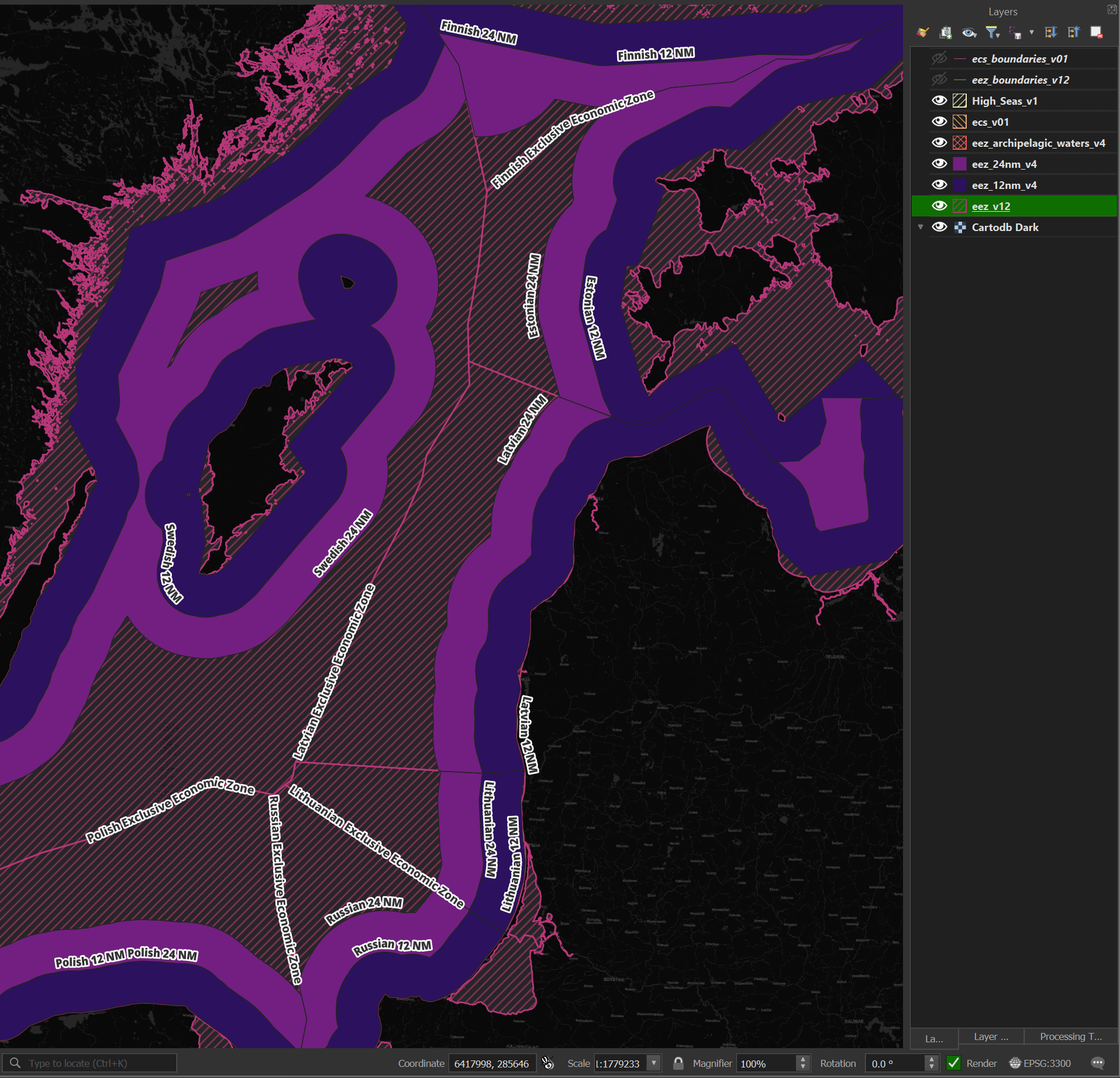
Marine Regions has GeoPackage files delineating maritime boundaries. Seven of the nine files contain polygons that I'll use to determine the waters a given image's centroid is in.
$ cd ~/marineregions_org
$ ls -lh *.gpkg
..  69M .. eez_12nm_v4.gpkg
..  60M .. eez_24nm_v4.gpkg
..  77M .. eez_internal_waters_v4.gpkg
..  16M .. eez_boundaries_v12.gpkg
.. 157M .. eez_v12.gpkg
..  39M .. eez_archipelagic_waters_v4.gpkg
.. 2.1M .. ecs_boundaries_v01.gpkg
.. 7.0M .. ecs_v01.gpkg
.. 8.8M .. High_Seas_v1.gpkg
Below is a rendering of this dataset around the Baltic Sea.
I'll run the following to import the GeoPackage files into DuckDB.
$ for FILENAME in *.gpkg; do
      BASENAME=`echo "$FILENAME" | cut -d. -f1`
      ~/duckdb -c "CREATE OR REPLACE TABLE $BASENAME AS
                      SELECT *
                      FROM   ST_READ('$FILENAME');" \
          ~/capella.duckdb
  done
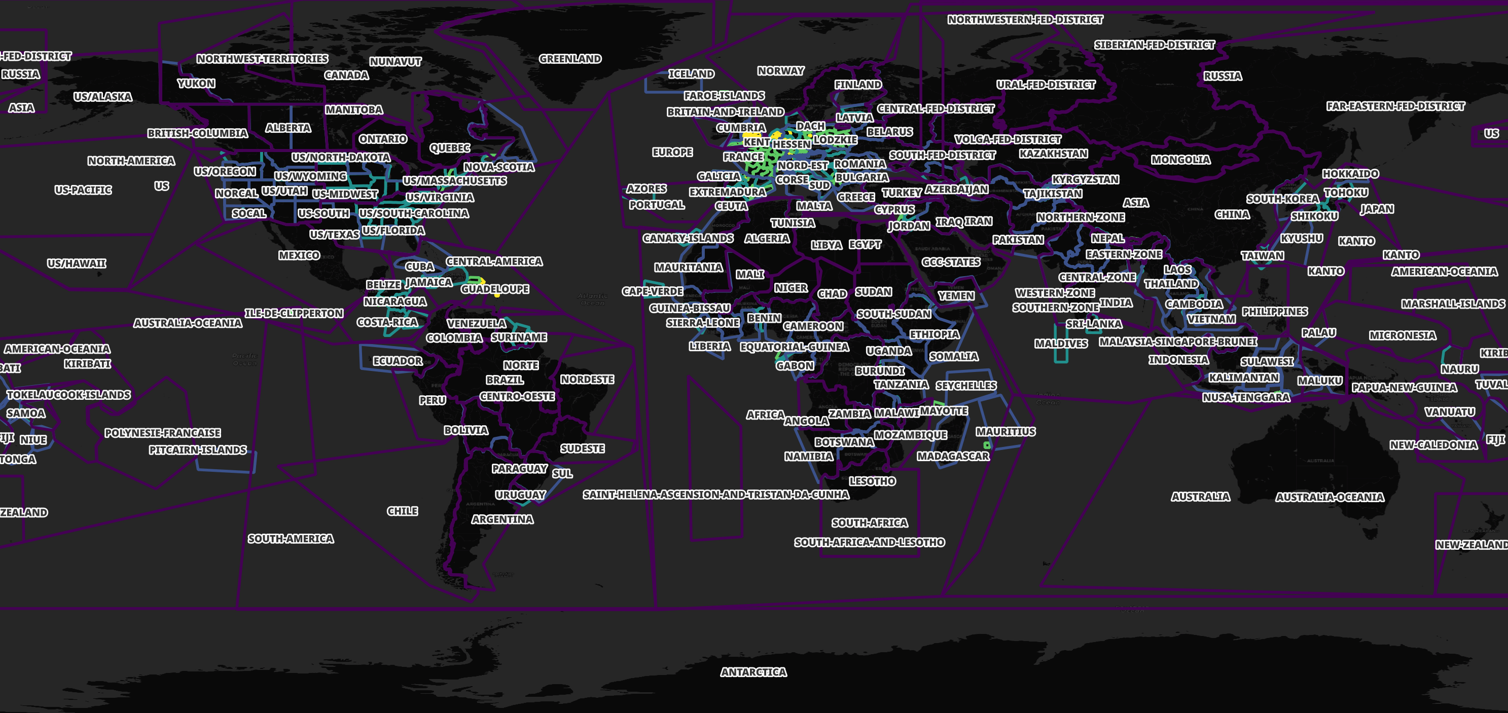
GeoFabrik's OSM Partitions
GeoFabrik publishes a GeoJSON file that shows all of the spatial partitions they use for their OpenStreetMap (OSM) releases.
$ wget -O ~/geofabrik.geojson \
    https://download.geofabrik.de/index-v1.json
Below is an example record. I've excluded the geometry field for readability.
$ jq -S '.features[0]' ~/geofabrik.geojson \
    | jq 'del(.geometry)'
{
  "properties": {
    "id": "afghanistan",
    "iso3166-1:alpha2": [
      "AF"
    ],
    "name": "Afghanistan",
    "parent": "asia",
    "urls": {
      "bz2": "https://download.geofabrik.de/asia/afghanistan-latest.osm.bz2",
      "history": "https://osm-internal.download.geofabrik.de/asia/afghanistan-internal.osh.pbf",
      "pbf": "https://download.geofabrik.de/asia/afghanistan-latest.osm.pbf",
      "pbf-internal": "https://osm-internal.download.geofabrik.de/asia/afghanistan-latest-internal.osm.pbf",
      "shp": "https://download.geofabrik.de/asia/afghanistan-latest-free.shp.zip",
      "taginfo": "https://taginfo.geofabrik.de/asia:afghanistan",
      "updates": "https://download.geofabrik.de/asia/afghanistan-updates"
    }
  },
  "type": "Feature"
}
These partitions cover anywhere with a landmass on Earth.
I'll import GeoFabrik's spatial partitions into DuckDB.
$ ~/duckdb ~/capella.duckdb
CREATE OR REPLACE TABLE geofabrik AS
    SELECT * EXCLUDE(urls),
           REPLACE(urls::JSON->'$.pbf', '"', '') AS url
    FROM ST_READ('/home/mark/geofabrik.geojson');
Below I'll list out all of the partitions and their corresponding PBF URLs containing OSM data for Monaco.
SELECT   id,
         url
FROM     geofabrik
WHERE    ST_CONTAINS(geom, ST_POINT(7.4210967, 43.7340769))
ORDER BY ST_AREA(geom);
┌────────────────────────────┬───────────────────────────────────────────────────────────────────────────────────────┐
│             id             │                                          url                                          │
│          varchar           │                                        varchar                                        │
├────────────────────────────┼───────────────────────────────────────────────────────────────────────────────────────┤
│ monaco                     │ https://download.geofabrik.de/europe/monaco-latest.osm.pbf                            │
│ provence-alpes-cote-d-azur │ https://download.geofabrik.de/europe/france/provence-alpes-cote-d-azur-latest.osm.pbf │
│ alps                       │ https://download.geofabrik.de/europe/alps-latest.osm.pbf                              │
│ france                     │ https://download.geofabrik.de/europe/france-latest.osm.pbf                            │
│ europe                     │ https://download.geofabrik.de/europe-latest.osm.pbf                                   │
└────────────────────────────┴───────────────────────────────────────────────────────────────────────────────────────┘
Some areas have more than one file covering their geometry. This allows for downloading smaller files if you're only interested in a certain location or a larger file if you want to explore a larger area. Western Europe is heavily partitioned as shown below.
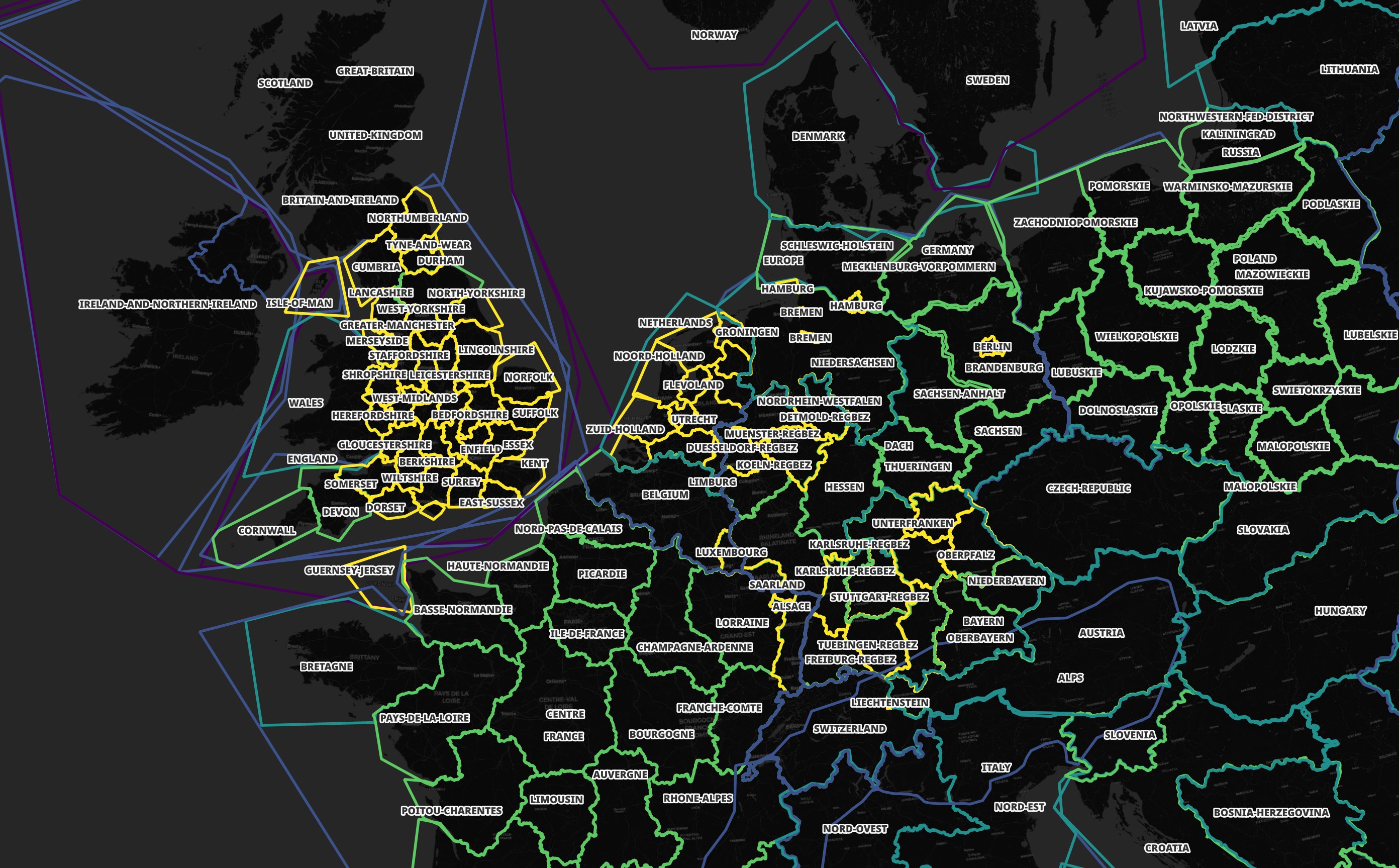
I'll use these partitions to better identify the regions of the world that Capella's images are in.
Capella's Deliverables
The data folder has a YYYY/M/D/<task> hierarchy for when a task's imagery was captured. Within any one task's folder, there can be between one and six imagery deliverables. These six deliverable types are in either CPHC, NITF or GeoTIFF format. There is also a JSON-formatted metadata file.
Below are some example filenames and typical file sizes.
Size | Filename
-----|------------------------------------------------------------------
1.2G | CAPELLA_C06_SM_CPHD_HH_20240205150941_20240205150944.cphd
698M | CAPELLA_C02_SP_SICD_HH_20201201165028_20201201165030.ntf
179M | CAPELLA_C06_SS_SIDD_HH_20240220102017_20240220102030.ntf
147M | CAPELLA_C06_SS_GEO_HH_20230607164219_20230607164233.tif
113K | CAPELLA_C06_SS_GEO_HH_20230607164219_20230607164233_extended.json
The naming convention is CAPELLA_<satellite number>_<imaging mode>_<instrument mode>_<polarisation>_<start time>_<end time>.<file format>.
Compensated Phase History Data
The first file format is Compensated Phase History Data (CPHD). These contain the lowest-level data. The files themselves can't be opened natively by QGIS or ArcGIS Pro. Below I'll extract the metadata from a CPHD file using sarpy.
$ python3
import json

from   sarpy.io.phase_history.converter import open_phase_history


reader = open_phase_history('CAPELLA_C06_SM_CPHD_HH_20240205150941_20240205150944.cphd')
open('CPHD_metadata.json', 'w')\
    .write(json.dumps(reader.cphd_details.cphd_meta.to_dict(),
                      sort_keys=True,
                      indent=4))
The above produced a 770-line JSON file. Below are the top-level keys.
$ jq -S 'keys' CPHD_metadata.json
[
  "Antenna",
  "Channel",
  "CollectionID",
  "Data",
  "Dwell",
  "Global",
  "PVP",
  "ReferenceGeometry",
  "SceneCoordinates",
  "TxRcv"
]
Below is the reference geometry from this image.
$ jq -S '.ReferenceGeometry' CPHD_metadata.json
{
  "Monostatic": {
    "ARPPos": {
      "X": 4701106.254980212,
      "Y": 959808.696687446,
      "Z": 4797224.220362454
    },
    "ARPVel": {
      "X": -4035.1181836278365,
      "Y": 5476.740806967509,
      "Z": 2842.3782662611957
    },
    "AzimuthAngle": 145.62754627711047,
    "DopplerConeAngle": 90.08471452924621,
    "GrazeAngle": 61.93658813756064,
    "GroundRange": 205072.24957530506,
    "IncidenceAngle": 28.06341186243936,
    "LayoverAngle": 145.7899079199028,
    "SideOfTrack": "L",
    "SlantRange": 466718.55376981717,
    "SlopeAngle": 61.9366836380116,
    "TwistAngle": -0.14327245798833665
  },
  "ReferenceTime": 1.6286937367274126,
  "SRP": {
    "ECF": {
      "X": 4314829.959742774,
      "Y": 765392.335750063,
      "Z": 4621670.494197229
    },
    "IAC": {
      "X": 0,
      "Y": 0,
      "Z": 0
    }
  },
  "SRPCODTime": 1.6286937698259407,
  "SRPDwellTime": 1.5222835344626993
}
Sensor-Independent Derived Data
The second file format is Sensor-Independent Derived Data (SIDD). This file includes coordinate and product image pixel array data. These files can be opened by both QGIS and ArcGIS Pro natively.
$ python3
import json

from   sarpy.io.product.converter import open_product


reader = open_product('CAPELLA_C06_SS_SIDD_HH_20240220102017_20240220102030.ntf')

open('SIDD_metadata.json', 'w')\
    .write(json.dumps(reader.get_sidds_as_tuple()[0].to_dict(),
                      sort_keys=True,
                      indent=4))
The above produced 652 lines of JSON.
$ jq -S 'keys' SIDD_metadata.json
[
  "Display",
  "ExploitationFeatures",
  "GeoData",
  "Measurement",
  "ProductCreation",
  "Radiometric"
]
Below is a rich amount of imagery collection details.
$ jq -S '.ExploitationFeatures.Collections' SIDD_metadata.json
[
  {
    "Information": {
      "CollectionDateTime": "2024-02-20T10:20:24.365349Z",
      "CollectionDuration": 12.216860464,
      "RadarMode": {
        "ModeType": "DYNAMIC STRIPMAP"
      },
      "SensorName": "capella-6"
    },
    "identifier": "20FEB24capella-6102018"
  }
]
Sensor-Independent Complex Data
The third file format is Sensor-Independent Complex Data (SCID). These files have SAR imagery that was processed through an image formation algorithm and are less idiosyncratic than CPHD. These files can be opened by both QGIS and ArcGIS Pro natively. Below I'll extract the metadata from an SCID file using sarpy.
$ python3
import json

from   sarpy.io.complex.converter import open_complex


reader = open_complex('CAPELLA_C02_SP_SICD_HH_20201201165028_20201201165030.ntf')
open('SICD_metadata.json', 'w')\
    .write(json.dumps(reader.get_sicds_as_tuple()[0].to_dict(),
                      sort_keys=True,
                      indent=4))
The above produced 1,611 lines of JSON. Below are the top-level keys.
$ jq -S 'keys' SICD_metadata.json
[
  "Antenna",
  "CollectionInfo",
  "GeoData",
  "Grid",
  "ImageCreation",
  "ImageData",
  "ImageFormation",
  "Position",
  "RMA",
  "RadarCollection",
  "Radiometric",
  "SCPCOA",
  "Timeline"
]
These are the satellite's locations as it took 4 captures that produced the final image.
$ jq -c '.GeoData.ValidData[]' SICD_metadata.json
{"Lat":14.185359809181293,"Lon":38.76800329637501,"index":1}
{"Lat":14.135856042457226,"Lon":38.81669669505986,"index":2}
{"Lat":14.103769536839271,"Lon":38.78382371069954,"index":3}
{"Lat":14.151016403993216,"Lon":38.73282983999779,"index":4}
Below are the processing steps this image went through.
$ jq -S '.ImageFormation.Processings' SICD_metadata.json
[
  {
    "Applied": true,
    "Type": "Backprojected to DEM"
  }
]
Task Metadata
The fourth file type is a JSON-formatted metadata file. These contain a large amount of information about where and how the image was captured.
Below I'll enrich the metadata in these files with the other datasets I've downloaded. As of this writing, I haven't been able to extract the centroids from Capella's Slant Plane or PFA imagery. I'll revisit this if this post proves to be popular.
$ cd ~/capella
$ vi enrich.py
from   datetime         import datetime
import json
from   pathlib          import Path

import duckdb
import pyproj
from   rich.progress    import track
from   shapely          import wkt
from   shapely.geometry import shape, Point
from   shapely.ops      import transform


waters_tables = (
    'High_Seas_v1',
    'eez_archipelagic_waters_v4',
    'ecs_boundaries_v01',
    'eez_boundaries_v12',
    'ecs_v01',
    'eez_internal_waters_v4',
    'eez_12nm_v4',
    'eez_v12',
    'eez_24nm_v4')

con = duckdb.connect(database='/home/mark/capella.duckdb')
df = con.sql('INSTALL spatial;')

with open('enriched.json', 'w') as f:
    for filename in track(list(Path('.').glob('data/**/*_extended.json'))):
        (_,
         sat_num,
         imaging_mode,
         instrument_mode,
         polarisation,
         start,
         finish,
         _) = str(filename)\
                .split('/')[-1]\
                .split('.')[0]\
                .split('_')

        start = datetime.strptime(start, "%Y%m%d%H%M%S")\
                    .strftime("%Y-%m-%d %H:%M:%S")
        finish = datetime.strptime(finish, "%Y%m%d%H%M%S")\
                        .strftime("%Y-%m-%d %H:%M:%S")

        rec = json.loads(open(filename, 'r').read())

        out = {'filename':        str(filename),
               'num_bytes':       Path(filename).stat().st_size,
               'sat_num':         sat_num,
               'imaging_mode':    imaging_mode,
               'instrument_mode': instrument_mode,
               'polarisation':    polarisation,
               'start':           start,
               'finish':          finish,
               'ground_range_resolution':
                    rec['collect']['image']['ground_range_resolution'],
               'azimuth_looks':
                    rec['collect']['image']['azimuth_looks']}

        if  rec['collect']['image']['image_geometry']['type'] not in \
            ('slant_plane', 'pfa'):
            crs_ = pyproj.Proj(rec['collect']
                               ['image']
                               ['image_geometry']
                               ['coordinate_system']
                               ['wkt']).crs

            project = pyproj.Transformer.from_crs(
                crs_,
                pyproj.CRS('EPSG:4326'),
                always_xy=True).transform

            lon, _, _, lat, _, _ = rec['collect']\
                                      ['image']\
                                      ['image_geometry']\
                                      ['geotransform']
            point = transform(project, wkt.loads('POINT(%s %s)' % (lon, lat)))

            out['lon']  = point.x
            out['lat']  = point.y
            out['epsg'] = crs_.to_epsg()

            # Get waters
            for table in waters_tables:
                df = con.sql("""LOAD   spatial;
                                SELECT *
                                FROM   """ + table + """
                                WHERE  ST_CONTAINS(geom, ST_POINT(?, ?));""",
                             params=(point.x, point.y)).to_df()

                if not df.empty:
                    out['waters'] = json.loads(df.to_json())['GEONAME']['0']
                    break

            # Get GeoFabrik
            df = con.sql("""LOAD   spatial;
                            SELECT *
                            FROM   geofabrik
                            WHERE  ST_CONTAINS(geom, ST_POINT(?, ?))
                            ORDER BY ST_AREA(geom)
                            LIMIT 1;""",
                         params=(point.x, point.y)).to_df()

            if not df.empty:
                out['geofabrik'] = json.loads(df.to_json())['id']['0']

        f.write(json.dumps(out, sort_keys=True) + '\n')
$ python enrich.py
The above produced 834 enriched records, one for each tasking event. Below is an example record.
$ head -n1 enriched.json | jq -S .
{
  "epsg": 32637,
  "filename": "data/2020/12/1/CAPELLA_C02_SP_GEC_HH_20201201165018_20201201165040/CAPELLA_C02_SP_GEC_HH_20201201165018_20201201165040_extended.json",
  "finish": "2020-12-01 16:50:40",
  "geofabrik": "ethiopia",
  "imaging_mode": "SP",
  "instrument_mode": "GEC",
  "lat": 14.194039830026993,
  "lon": 38.72554635135875,
  "num_bytes": 141568,
  "polarisation": "HH",
  "sat_num": "C02",
  "start": "2020-12-01 16:50:18"
}
I'll import these records into DuckDB.
$ ~/duckdb ~/capella.duckdb
CREATE OR REPLACE TABLE capella AS
    SELECT *
    FROM READ_JSON('enriched.json');
Geo-Ellipsoid Corrected Data
The remaining deliverables are all formatted as GeoTiff files. They are called Single Look Complex (SLC), Geocoded Ellipsoid Corrected (GEC) and Geocoded Terrain Corrected (GEO). These files can be opened by both QGIS and ArcGIS Pro natively.
The GEC files Capella delivers are Cloud-Optimised GeoTIFF containers. These files contain Tiled Multi-Resolution TIFFs / Tiled Pyramid TIFFs. This means there are several versions of the same image at different resolutions within the TIFF file.
These files are structured so it's easy to only read a portion of a file for any one resolution you're interested in. A file might be 100 MB but a JavaScript-based Web Application might only need to download 2 MB of data from that file in order to render its lowest resolution.
Below I'll write a parser to convert the output from tiffinfo into JSON for each GEC file and include its corresponding satellite metadata.
$ python3
from   datetime      import datetime
import json
from   pathlib       import Path
import re
from   shlex         import quote
import sys

from   rich.progress import track
from   shpyx         import run as execute


def parse_tiff(lines:list):
    out, stack_id = {}, None

    for line in lines:
        if not stack_id:
            stack_id = 1
        elif line.startswith('TIFF Directory'):
            stack_id = stack_id + 1
        elif line.startswith('  ') and line.count(':') == 1:
            if stack_id not in out:
                out[stack_id] = {'stack_num': stack_id}

            x, y = line.strip().split(':')

            if len(x) > 1 and not x.startswith('Tag ') and \
               y and \
               len(str(y).strip()) > 1:
                out[stack_id][x.strip()] = y.strip()
        elif line.startswith('  ') and \
             line.count(':') == 2 and \
             'Image Width' in line:
            if stack_id not in out:
                out[stack_id] = {'stack_num': stack_id}

            _, width, _, _, _ = re.split(r'\: ([0-9]*)', line)
            out[stack_id]['width'] = int(width.strip())

    return [y for x, y in out.items()]


with open('geotiffs.json', 'w') as f:
    for path in track(list(Path('.').glob('data/**/*[0-9].tif'))):
        lines = execute('tiffinfo -i %s' % quote(path.absolute().as_posix()))\
                    .stdout\
                    .strip()\
                    .splitlines()

        try:
            sat_meta = json.loads(open(list(Path(path.parent)
                                                .rglob('*.json'))[0], 'r')
                                    .read())
        except:
            sat_meta = {}

        (_,
         sat_num,
         imaging_mode,
         instrument_mode,
         polarisation,
         start,
         finish) = str(path)\
                    .split('/')[-1]\
                    .split('.')[0]\
                    .split('_')

        start = datetime.strptime(start, "%Y%m%d%H%M%S")\
                    .strftime("%Y-%m-%d %H:%M:%S")
        finish = datetime.strptime(finish, "%Y%m%d%H%M%S")\
                        .strftime("%Y-%m-%d %H:%M:%S")

        for line in parse_tiff(lines):
            f.write(json.dumps({**line,
                                **{'filename': path.absolute().as_posix(),
                                   'sat_meta': sat_meta,
                                   'sat_num':         sat_num,
                                   'imaging_mode':    imaging_mode,
                                   'instrument_mode': instrument_mode,
                                   'polarisation':    polarisation,
                                   'start':           start,
                                   'finish':          finish}},
                               sort_keys=True) + '\n')
Below is an example record that was produced by the above script. There is one record for each stack / image in each GeoTIFF file.
$ head -n1 geotiffs.json \
    | jq -S 'del(.sat_meta)'
{
  "Bits/Sample": "32",
  "Compression Scheme": "AdobeDeflate",
  "Photometric Interpretation": "min-is-black",
  "Planar Configuration": "single image plane",
  "Predictor": "none 1 (0x1)",
  "Sample Format": "complex signed integer",
  "Software": "Capella SAR Processor (2.49.0, d0aa2ee3ad51f696b05db72f6705afc6e05000ec-dirty)",
  "filename": "/mnt/f/capella/data/2020/12/1/CAPELLA_C02_SP_SLC_HH_20201201165028_20201201165030/CAPELLA_C02_SP_SLC_HH_20201201165028_20201201165030.tif",
  "finish": "2020-12-01 16:50:30",
  "imaging_mode": "SP",
  "instrument_mode": "SLC",
  "polarisation": "HH",
  "sat_num": "C02",
  "stack_num": 1,
  "start": "2020-12-01 16:50:28",
  "width": 9945
}
I'll load the JSON into a DuckDB table.
$ ~/duckdb ~/capella.duckdb
CREATE OR REPLACE TABLE geotiffs AS
    SELECT *
    FROM   READ_JSON('geotiffs.json');
Below are the image counts broken down by the stack number and satellite.
WITH a AS (
    SELECT stack_num,
           sat_num
    FROM   geotiffs
)
PIVOT    a
ON       stack_num
USING    COUNT(*)
GROUP BY sat_num
ORDER BY sat_num;
┌─────────┬───────┬───────┬───────┬───────┬───────┬───────┬───────┬───────┬───────┐
│ sat_num │   1   │   2   │   3   │   4   │   5   │   6   │   7   │   8   │   9   │
│ varchar │ int64 │ int64 │ int64 │ int64 │ int64 │ int64 │ int64 │ int64 │ int64 │
├─────────┼───────┼───────┼───────┼───────┼───────┼───────┼───────┼───────┼───────┤
│ C02     │    39 │    38 │    38 │    38 │    38 │    38 │     4 │     0 │     0 │
│ C03     │    16 │    16 │    16 │    16 │    16 │    16 │     2 │     0 │     0 │
│ C05     │    10 │    10 │    10 │    10 │    10 │    10 │     0 │     0 │     0 │
│ C06     │    96 │    69 │    69 │    69 │    69 │    63 │    10 │     4 │     2 │
│ C07     │     3 │     2 │     2 │     2 │     2 │     2 │     2 │     2 │     0 │
│ C08     │    42 │    30 │    30 │    30 │    30 │    30 │     6 │     2 │     0 │
│ C09     │    71 │    47 │    47 │    47 │    47 │    45 │     1 │     1 │     0 │
│ C10     │    57 │    38 │    38 │    38 │    38 │    34 │     0 │     0 │     0 │
│ C11     │     9 │     6 │     6 │     6 │     6 │     6 │     0 │     0 │     0 │
│ C14     │    12 │     8 │     8 │     8 │     8 │     8 │     0 │     0 │     0 │
├─────────┴───────┴───────┴───────┴───────┴───────┴───────┴───────┴───────┴───────┤
│ 10 rows                                                              10 columns │
└─────────────────────────────────────────────────────────────────────────────────┘
Below are the image width buckets and stack counts. I find it odd that the wider images tend to use fewer stacks.
WITH a AS (
    SELECT stack_num,
           (ROUND(width / 10000) * 10000)::INT AS width
    FROM   geotiffs
)
PIVOT    a
ON       stack_num
USING    COUNT(*)
GROUP BY width
ORDER BY width;
┌────────┬───────┬───────┬───────┬───────┬───────┬───────┬───────┬───────┬───────┐
│ width  │   1   │   2   │   3   │   4   │   5   │   6   │   7   │   8   │   9   │
│ int32  │ int64 │ int64 │ int64 │ int64 │ int64 │ int64 │ int64 │ int64 │ int64 │
├────────┼───────┼───────┼───────┼───────┼───────┼───────┼───────┼───────┼───────┤
│      0 │     3 │     0 │    40 │   253 │   261 │   252 │    25 │     9 │     2 │
│  10000 │    97 │   246 │   219 │     9 │     3 │     0 │     0 │     0 │     0 │
│  20000 │   141 │    11 │     2 │     2 │     0 │     0 │     0 │     0 │     0 │
│  30000 │   101 │     2 │     3 │     0 │     0 │     0 │     0 │     0 │     0 │
│  40000 │     2 │     2 │     0 │     0 │     0 │     0 │     0 │     0 │     0 │
│  50000 │     6 │     0 │     0 │     0 │     0 │     0 │     0 │     0 │     0 │
│  60000 │     0 │     3 │     0 │     0 │     0 │     0 │     0 │     0 │     0 │
│  70000 │     2 │     0 │     0 │     0 │     0 │     0 │     0 │     0 │     0 │
│ 120000 │     3 │     0 │     0 │     0 │     0 │     0 │     0 │     0 │     0 │
└────────┴───────┴───────┴───────┴───────┴───────┴───────┴───────┴───────┴───────┘
Below are the image width buckets by satellite number.
WITH a AS (
    SELECT sat_num,
           (ROUND(width / 10000) * 10000)::INT AS width
    FROM   geotiffs
)
PIVOT    a
ON       sat_num
USING    COUNT(*)
GROUP BY width
ORDER BY width;
┌────────┬───────┬───────┬───────┬───────┬───────┬───────┬───────┬───────┬───────┬───────┐
│ width  │  C02  │  C03  │  C05  │  C06  │  C07  │  C08  │  C09  │  C10  │  C11  │  C14  │
│ int32  │ int64 │ int64 │ int64 │ int64 │ int64 │ int64 │ int64 │ int64 │ int64 │ int64 │
├────────┼───────┼───────┼───────┼───────┼───────┼───────┼───────┼───────┼───────┼───────┤
│      0 │   118 │    54 │    30 │   222 │    10 │   103 │   147 │   117 │    20 │    24 │
│  10000 │    73 │    28 │    20 │   154 │     4 │    67 │   111 │    85 │    12 │    20 │
│  20000 │    22 │    16 │    10 │    29 │     1 │    26 │    20 │    23 │     5 │     4 │
│  30000 │    18 │     0 │     0 │    32 │     2 │     4 │    26 │    18 │     2 │     4 │
│  40000 │     0 │     0 │     0 │     4 │     0 │     0 │     0 │     0 │     0 │     0 │
│  50000 │     2 │     0 │     0 │     4 │     0 │     0 │     0 │     0 │     0 │     0 │
│  60000 │     0 │     0 │     0 │     2 │     0 │     0 │     1 │     0 │     0 │     0 │
│  70000 │     0 │     0 │     0 │     2 │     0 │     0 │     0 │     0 │     0 │     0 │
│ 120000 │     0 │     0 │     0 │     2 │     0 │     0 │     1 │     0 │     0 │     0 │
└────────┴───────┴───────┴───────┴───────┴───────┴───────┴───────┴───────┴───────┴───────┘
There isn't any variation in their compression schemes.
WITH a AS (
    SELECT "Compression Scheme" AS cs,
           sat_num
    FROM   geotiffs
)
PIVOT    a
ON       cs
USING    COUNT(*)
GROUP BY sat_num
ORDER BY sat_num;
┌─────────┬──────────────┐
│ sat_num │ AdobeDeflate │
│ varchar │    int64     │
├─────────┼──────────────┤
│ C02     │          233 │
│ C03     │           98 │
│ C05     │           60 │
│ C06     │          451 │
│ C07     │           17 │
│ C08     │          200 │
│ C09     │          306 │
│ C10     │          243 │
│ C11     │           39 │
│ C14     │           52 │
├─────────┴──────────────┤
│ 10 rows      2 columns │
└────────────────────────┘
Every GeoTIFF file from Capella has its metadata from the satellite's capture and processing embedded within it. So even without the counterpart metadata JSON file, everything about it's tasking is self-contained.
$ gdalinfo -json data/2020/12/1/CAPELLA_C02_SP_SLC_HH_20201201165028_20201201165030/CAPELLA_C02_SP_SLC_HH_20201201165028_20201201165030.tif \
    | jq -S .metadata['""'].TIFFTAG_IMAGEDESCRIPTION \
    | jq -S '. | fromjson | del(.collect)'
{
  "copyright": "Copyright 2023 Capella Space. All Rights Reserved.",
  "license": "https://www.capellaspace.com/data-licensing/",
  "processing_deployment": "production",
  "processing_time": "2023-10-21T11:39:13.474724Z",
  "product_type": "SLC",
  "product_version": "1.10",
  "software_revision": "d0aa2ee3ad51f696b05db72f6705afc6e05000ec-dirty",
  "software_version": "2.49.0"
}
$ gdalinfo -json data/2020/12/1/CAPELLA_C02_SP_SLC_HH_20201201165028_20201201165030/CAPELLA_C02_SP_SLC_HH_20201201165028_20201201165030.tif \
    | jq -S .metadata['""'].TIFFTAG_IMAGEDESCRIPTION \
    | jq -S '. | fromjson | .collect | keys'
[
  "collect_id",
  "image",
  "local_datetime",
  "local_timezone",
  "mode",
  "platform",
  "pointing",
  "radar",
  "receive_antenna",
  "start_timestamp",
  "state",
  "stop_timestamp",
  "transmit_antenna"
]
Modes & Polarisation
SAR radar beams can switch between horizontal and vertical polarisation both when sending and receiving. These are denoted by two letters. For example: HV would mean horizontal transmission and vertical receiving.
Horizontal polarisation is ideal for flat and low surfaces, like rivers, bridges and power lines. Vertical polarisation is ideal for buildings, rough seas and transmission towers.
The majority of tasks in Capella's Open Data Feed use horizontal polarisation.
$ ~/duckdb ~/capella.duckdb
SELECT   imaging_mode,
         instrument_mode,
         polarisation,
         COUNT(*)
FROM     capella
GROUP BY 1, 2, 3
ORDER BY 4 DESC;
┌──────────────┬─────────────────┬──────────────┬──────────────┐
│ imaging_mode │ instrument_mode │ polarisation │ count_star() │
│   varchar    │     varchar     │   varchar    │    int64     │
├──────────────┼─────────────────┼──────────────┼──────────────┤
│ SP           │ GEO             │ HH           │          159 │
│ SP           │ GEC             │ HH           │          158 │
│ SM           │ GEO             │ HH           │           68 │
│ SM           │ GEC             │ HH           │           67 │
│ SS           │ GEC             │ HH           │           39 │
│ SS           │ GEO             │ HH           │           39 │
│ SM           │ GEO             │ VV           │            7 │
│ SM           │ GEC             │ VV           │            7 │
│ SP           │ GEO             │ VV           │            4 │
│ SP           │ GEC             │ VV           │            4 │
│ SS           │ GEO             │ VV           │            2 │
│ SS           │ GEC             │ VV           │            2 │
├──────────────┴─────────────────┴──────────────┴──────────────┤
│ 12 rows                                            4 columns │
└──────────────────────────────────────────────────────────────┘
Resolutions and Looks
SAR imagery can take multiple 'looks' at a location when capturing an image. Most of the imagery in this feed either takes either a single look, five looks or nine looks. Generally, the more looks, the finer the resolution of the final image.
Most of the imagery is around the 50-cm resolution though there are some images 32-cm images as well.
WITH a AS (
    SELECT (ROUND(ROUND(ground_range_resolution * 100) / 10) * 10)::INT AS cm_res,
           printf('%02d', azimuth_looks::INT) AS azimuth_looks
    FROM   capella
)
PIVOT    a
ON       azimuth_looks
USING    COUNT(*)
GROUP BY cm_res
ORDER BY cm_res;
┌────────┬───────┬───────┬───────┬───────┬───────┬───────┬───────┐
│ cm_res │  01   │  02   │  05   │  08   │  09   │  10   │  11   │
│ int32  │ int64 │ int64 │ int64 │ int64 │ int64 │ int64 │ int64 │
├────────┼───────┼───────┼───────┼───────┼───────┼───────┼───────┤
│     30 │     2 │     0 │     0 │     0 │     0 │     0 │     0 │
│     40 │    73 │     0 │     0 │     0 │     0 │     0 │     0 │
│     50 │    60 │     0 │     0 │     0 │    18 │     2 │     0 │
│     60 │    22 │     0 │     0 │     2 │   143 │     2 │     0 │
│     70 │    23 │     0 │     0 │     0 │    85 │     2 │     2 │
│     80 │    13 │     0 │     6 │     0 │    49 │     0 │     0 │
│     90 │    21 │     0 │    12 │     0 │     6 │     0 │     0 │
│    100 │     6 │     2 │    16 │     0 │     6 │     0 │     0 │
│    110 │    12 │     0 │    16 │     0 │     4 │     0 │     0 │
│    120 │    17 │     0 │    12 │     0 │     2 │     0 │     0 │
│    130 │    18 │     0 │    10 │     0 │     0 │     0 │     0 │
│    140 │    21 │     0 │    10 │     0 │     0 │     0 │     0 │
│    150 │    45 │     0 │     0 │     0 │     0 │     0 │     0 │
│    160 │    23 │     0 │     0 │     0 │     0 │     0 │     0 │
│    170 │    15 │     0 │     0 │     0 │     0 │     0 │     0 │
│    180 │    10 │     0 │     0 │     0 │     0 │     0 │     0 │
│    190 │    20 │     0 │     0 │     0 │     0 │     0 │     0 │
│    200 │    14 │     0 │     0 │     0 │     0 │     0 │     0 │
│    210 │     2 │     0 │     0 │     0 │     0 │     0 │     0 │
│    220 │     1 │     0 │     0 │     0 │     0 │     0 │     0 │
│    260 │     4 │     0 │     0 │     0 │     0 │     0 │     0 │
│    310 │     2 │     0 │     0 │     0 │     0 │     0 │     0 │
│    380 │     1 │     0 │     0 │     0 │     0 │     0 │     0 │
│    550 │     2 │     0 │     0 │     0 │     0 │     0 │     0 │
├────────┴───────┴───────┴───────┴───────┴───────┴───────┴───────┤
│ 24 rows                                              8 columns │
└────────────────────────────────────────────────────────────────┘
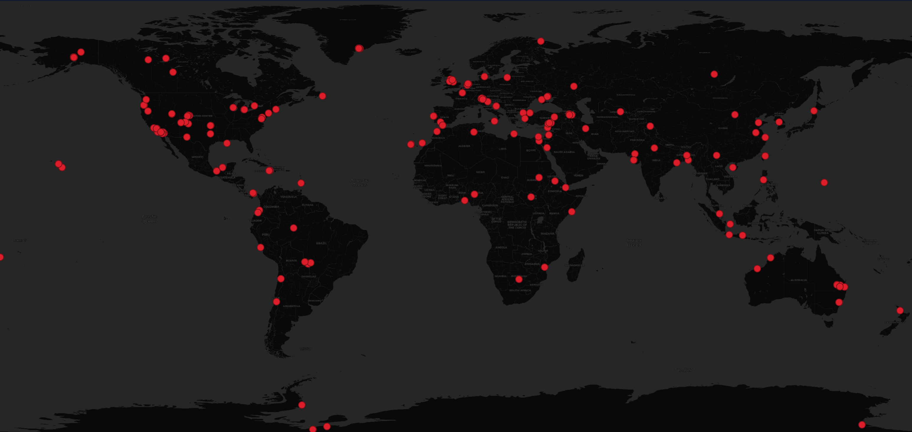
Geography
Below are the locations of the non-slant-plane and PFA imagery.
$ ~/duckdb ~/capella.duckdb
COPY (
    SELECT ST_POINT(lon,lat)::GEOMETRY AS geom
    FROM   capella
    WHERE  lon AND lat
) TO 'capella.gpkg'
  WITH (FORMAT GDAL,
        DRIVER 'GPKG',
        LAYER_CREATION_OPTIONS 'WRITE_BBOX=YES');
Below are the 25 most common GeoFabrik partitions found in Capella's Open Data Feed.
SELECT   geofabrik,
         COUNT(*)
FROM     capella
WHERE    geofabrik IS NOT NULL
GROUP BY 1
ORDER BY 2 DESC
LIMIT    25;
┌──────────────────┬──────────────┐
│    geofabrik     │ count_star() │
│     varchar      │    int64     │
├──────────────────┼──────────────┤
│ socal            │           52 │
│ andalucia        │           40 │
│ western-zone     │           28 │
│ us/alaska        │           28 │
│ turkey           │           26 │
│ greenland        │           24 │
│ australia        │           24 │
│ us/oregon        │           18 │
│ canary-islands   │           18 │
│ sudan            │           14 │
│ bangladesh       │           12 │
│ us/colorado      │           10 │
│ haiti-and-domrep │           10 │
│ pakistan         │           10 │
│ switzerland      │            9 │
│ nigeria          │            8 │
│ us/hawaii        │            8 │
│ us/michigan      │            8 │
│ antarctica       │            8 │
│ ukraine          │            8 │
│ portugal         │            6 │
│ armenia          │            6 │
│ mexico           │            6 │
│ isole            │            6 │
│ panama           │            5 │
├──────────────────┴──────────────┤
│ 25 rows               2 columns │
└─────────────────────────────────┘
Below are the 25 most common maritime locations of their imagery.
SELECT   waters,
         COUNT(*)
FROM     capella
WHERE    waters IS NOT NULL
GROUP BY 1
ORDER BY 2 DESC
LIMIT    25;
┌──────────────────────────────────┬──────────────┐
│              waters              │ count_star() │
│             varchar              │    int64     │
├──────────────────────────────────┼──────────────┤
│ Indian Internal Waters           │           28 │
│ Turkish 12 NM                    │           18 │
│ United States 12 NM (Hawaii)     │            6 │
│ Spanish 12 NM (Canary Islands)   │            5 │
│ United States 12 NM              │            4 │
│ Portuguese Internal Waters       │            4 │
│ Indonesian Archipelagic Waters   │            2 │
│ Syrian 12 NM                     │            2 │
│ Libyan 12 NM                     │            2 │
│ Croatian Internal Waters         │            2 │
│ Egyptian Exclusive Economic Zone │            2 │
│ Australian 12 NM                 │            2 │
│ Mexican Exclusive Economic Zone  │            2 │
│ Mexican 12 NM                    │            2 │
│ Australian Internal Waters       │            2 │
│ Chinese 12 NM                    │            2 │
│ Moroccan 12 NM                   │            2 │
│ Peruvian Internal Waters         │            2 │
│ Panamanian Internal Waters       │            2 │
│ Fijian Archipelagic Waters       │            2 │
│ Philippine Archipelagic Waters   │            2 │
│ Djiboutian Internal Waters       │            2 │
│ Saint Vincentian 12 NM           │            2 │
│ Danish 12 NM                     │            2 │
│ Bangladeshi Internal Waters      │            2 │
├──────────────────────────────────┴──────────────┤
│ 25 rows                               2 columns │
└─────────────────────────────────────────────────┘
Dates and Times
The oldest imagery in this feed is from the end of 2020. The uploads were pretty consistent up until this year where there was a gap of a few months where no imagery was uploaded into Capella's Open Data Feed S3 bucket.
WITH a AS (
    SELECT   strftime(start, '%Y') AS year,
             strftime(start, '%m') AS month
    FROM     capella
    ORDER BY start
)
PIVOT    a
ON       year
USING    COUNT(*)
GROUP BY month
ORDER BY month;
┌─────────┬───────┬───────┬───────┬───────┬───────┐
│  month  │ 2020  │ 2021  │ 2022  │ 2023  │ 2024  │
│ varchar │ int64 │ int64 │ int64 │ int64 │ int64 │
├─────────┼───────┼───────┼───────┼───────┼───────┤
│ 01      │     0 │    24 │     3 │     9 │    27 │
│ 02      │     0 │    54 │    27 │     9 │    30 │
│ 03      │     0 │    45 │    48 │    12 │     3 │
│ 04      │     0 │    39 │     9 │    12 │    27 │
│ 05      │     0 │    24 │     3 │    12 │     0 │
│ 06      │     0 │     6 │     6 │    27 │     0 │
│ 07      │     0 │    27 │     0 │    15 │     3 │
│ 08      │     0 │    30 │     3 │    15 │     2 │
│ 09      │     0 │    69 │     0 │    15 │     0 │
│ 10      │     0 │    12 │    66 │     9 │     0 │
│ 11      │     0 │    24 │     3 │    30 │     0 │
│ 12      │    16 │    27 │     0 │    12 │     0 │
├─────────┴───────┴───────┴───────┴───────┴───────┤
│ 12 rows                               6 columns │
└─────────────────────────────────────────────────┘