The Overture Maps Foundation is a joint development project that publishes global, open map data.
Finding global datasets, outside of OpenStreetMap (OSM), is challenging and when the datasets need to be free, the choices are even fewer and further between.
To add to that, OSM won't accept bulk submissions produced by AI; instead, they want every change to be confirmed by a human. Finding volunteers willing to validate 30K building height measurements from LiDAR scans can be far beyond the reach of charity.
But the world of GIS isn't about using a single data provider. GIS is an ecosystem. Using several datasets from a diverse and unaffiliated set of providers is the path to innovation. To add to this, maps are outdated the moment they're published and AI being fed data from an ever-increasing number of sensors will be key to shorter refresh intervals.
Overture aims to take data from a broad range of providers and blend them into Parquet files hosted on Cloud storage and refreshed every month.
The firms partnering with Overture include Amazon, Esri, Grab, Hyundai, Meta, Microsoft, Precisely, Tripadvisor and TomTom.
These firms have committed to providing funding, engineering and data. When providers are unwilling to publish proprietary datasets, there are cases where they'll use AI to produce derivative datasets.
Google aren't a part of the Overture Foundation but their open buildings dataset helps fill gaps in the map where OSM's and Microsoft's ML-generated buildings have failed to identify building footprints.
Overture is led by Marc Prioleau, who previously spent four years as the head of business development for Mapping and Location at Meta, five years at Mapbox, including sitting on their Board of Directors and a year at Uber doing business development for their location-based services.
With this week's latest release, Overture now has over 7 TB of GIS data hosted on S3.
In this post, I'll review some of the updates they've made in the past few months.
My Workstation
I'm using a 6 GHz Intel Core i9-14900K CPU. It has 8 performance cores and 16 efficiency cores with a total of 32 threads and 32 MB of L2 cache. It has a liquid cooler attached and is housed in a spacious, full-sized, Cooler Master HAF 700 computer case. I've come across videos on YouTube where people have managed to overclock the i9-14900KF to 9.1 GHz.
The system has 96 GB of DDR5 RAM clocked at 6,000 MT/s and a 5th-generation, Crucial T700 4 TB NVMe M.2 SSD which can read at speeds up to 12,400 MB/s. There is a heatsink on the SSD to help keep its temperature down. This is my system's C drive.
The system is powered by a 1,200-watt, fully modular, Corsair Power Supply and is sat on an ASRock Z790 Pro RS Motherboard.
I'm running Ubuntu 22 LTS via Microsoft's Ubuntu for Windows on Windows 11 Pro. In case you're wondering why I don't run a Linux-based desktop as my primary work environment, I'm still using an Nvidia GTX 1080 GPU which has better driver support on Windows and I use ArcGIS Pro from time to time which only supports Windows natively.
Installing Prerequisites
I'll use a few tools to help prepare and visualise the data in this post.
$ sudo apt update
$ sudo apt install \
    awscli \
    jq \
    python3-pip \
    python3-virtualenv
I'll set up a Python Virtual Environment and install some dependencies.
$ virtualenv ~/.overture
$ source ~/.overture/bin/activate
I've been working on a Parquet debugging tool. I'll use it to examine the results of Parquet compression in this post.
$ git clone https://github.com/marklit/pqview \
    ~/pqview
$ python3 -m pip install \
          -r ~/pqview/requirements.txt
I'll use DuckDB, along with its H3, JSON, Lindel, Parquet and Spatial extensions, in this post.
$ cd ~
$ wget -c https://github.com/duckdb/duckdb/releases/download/v1.1.3/duckdb_cli-linux-amd64.zip
$ unzip -j duckdb_cli-linux-amd64.zip
$ chmod +x duckdb
$ ~/duckdb
INSTALL h3 FROM community;
INSTALL lindel FROM community;
INSTALL json;
INSTALL parquet;
INSTALL spatial;
I'll set up DuckDB to load every installed extension each time it launches.
$ vi ~/.duckdbrc
.timer on
.width 180
LOAD h3;
LOAD lindel;
LOAD json;
LOAD parquet;
LOAD spatial;
The maps in this post were rendered with QGIS version 3.40. QGIS is a desktop application that runs on Windows, macOS and Linux. The application has grown in popularity in recent years and has ~15M application launches from users all around the world each month.
I used QGIS' Tile+ plugin to add geospatial context with Esri's World Imagery Basemap. The dark, non-satellite imagery maps are mostly made up of vector data from Natural Earth and Overture.
Political Boundaries
The Database of Global Administrative Areas (GADM) aims to map the administrative areas of all countries, at all levels of sub-division. Its records can be joined to Overture's and allow you to group them by continent, country and/or other political boundaries.
I'll download and import it into DuckDB. The following ZIP file is 1.4 GB and contains a GeoPackage (GPKG) file that is 2.6 GB. There are a total of 356,508 records.
$ wget -c https://geodata.ucdavis.edu/gadm/gadm4.1/gadm_410-gpkg.zip
$ unzip gadm_410-gpkg.zip

$ ~/duckdb ~/overture.duckdb
CREATE OR REPLACE TABLE gadm AS
    FROM   ST_READ('gadm_410.gpkg');
The DuckDB table has a disk footprint of 5 GB. Below is an example record.
$ echo "FROM  gadm
        WHERE NAME_2 = 'Tallinn'
        LIMIT 1" \
    | ~/duckdb -json ~/overture.duckdb \
    | jq -S .
[
  {
    "CC_1": "",
    "CC_2": "",
    "CC_3": "",
    "CC_4": "",
    "CC_5": "",
    "CONTINENT": "Europe",
    "COUNTRY": "Estonia",
    "DISPUTEDBY": "",
    "ENGTYPE_1": "County",
    "ENGTYPE_2": "Town",
    "ENGTYPE_3": "Administrative District",
    "ENGTYPE_4": "",
    "ENGTYPE_5": "",
    "GID_0": "EST",
    "GID_1": "EST.1_1",
    "GID_2": "EST.1.20_1",
    "GID_3": "EST.1.20.1_1",
    "GID_4": "",
    "GID_5": "",
    "GOVERNEDBY": "",
    "HASC_1": "EE.HA",
    "HASC_2": "EE.HA.TA",
    "HASC_3": "",
    "ISO_1": "",
    "NAME_0": "Estonia",
    "NAME_1": "Harju",
    "NAME_2": "Tallinn",
    "NAME_3": "Haabersti",
    "NAME_4": "",
    "NAME_5": "",
    "NL_NAME_1": "",
    "NL_NAME_2": "",
    "NL_NAME_3": "",
    "REGION": "",
    "SOVEREIGN": "Estonia",
    "SUBCONT": "",
    "TYPE_1": "Maakond",
    "TYPE_2": "Linn",
    "TYPE_3": "Linnaosa",
    "TYPE_4": "",
    "TYPE_5": "",
    "UID": 50179,
    "VALIDFR_1": "Unknown",
    "VALIDFR_2": "2002",
    "VALIDFR_3": "Unknown",
    "VALIDFR_4": "",
    "VARNAME_0": "",
    "VARNAME_1": "Harjumaa|Harju maakond",
    "VARNAME_2": "",
    "VARNAME_3": "",
    "VARNAME_4": "",
    "VARREGION": "",
    "geom": "MULTIPOLYGON (((24.62020123500008 59.38849636600014, ...)))"
  }
]
Natural Earth's Country Codes
GADM doesn't have two-letter ISO codes for identifying countries that line up well with what Overture use. For joins needing these, I'll use Natural Earth's dataset instead.
$ aws s3 cp \
        --no-sign-request \
        s3://naturalearth/10m_cultural/ne_10m_admin_0_countries_deu.zip \
        ~/
$ unzip ~/ne_10m_admin_0_countries_deu.zip \
        -d ~/ne_countries
Overture's List of Files
I'll download a JSON-formatted listing of every object in Overture's S3 bucket.
$ aws --no-sign-request \
      --output json \
      s3api \
      list-objects \
      --bucket overturemaps-us-west-2 \
      --max-items=1000000 \
    | jq -c '.Contents[]' \
    > overturemaps.s3.json
$ ~/duckdb ~/overture.duckdb
CREATE OR REPLACE TABLE s3 AS
    SELECT *,
           SPLIT(Key, '/')[1]                        AS section,
           SPLIT(Key, '/')[2]                        AS release,
           REPLACE(SPLIT(Key, '/')[3], 'theme=', '') AS theme,
           REPLACE(SPLIT(Key, '/')[4], 'type=', '')  AS theme_type
    FROM   READ_JSON('overturemaps.s3.json')
    WHERE  Key NOT LIKE '%planet%'
    AND    Key NOT LIKE '%_SUCCESS%'
    AND    Key NOT LIKE '%building-extracts%'
    AND    section = 'release';
Below are the release IDs, their weekday of release and size in GB. Releases are published in the middle of each month but there is a somewhat even distribution between them landing on Tuesdays, Wednesdays or Thursdays.
Overture's December release is 1.4x larger than April's release.
SELECT   release,
         strftime(release[:10]::DATE, '%a') week_day,
         ROUND(SUM(Size) / 1024 ** 3)::INT  sum_size
FROM     s3
GROUP BY 1
ORDER BY 1;
┌────────────────────┬──────────┬──────────┐
│      release       │ week_day │ sum_size │
│      varchar       │ varchar  │  int32   │
├────────────────────┼──────────┼──────────┤
│ 2023-07-26-alpha.0 │ Wed      │      201 │
│ 2023-10-19-alpha.0 │ Thu      │      326 │
│ 2023-11-14-alpha.0 │ Tue      │      296 │
│ 2023-12-14-alpha.0 │ Thu      │      353 │
│ 2024-01-17-alpha.0 │ Wed      │      356 │
│ 2024-02-15-alpha.0 │ Thu      │      355 │
│ 2024-03-12-alpha.0 │ Tue      │      356 │
│ 2024-04-16-beta.0  │ Tue      │      315 │
│ 2024-05-16-beta.0  │ Thu      │      413 │
│ 2024-06-13-beta.0  │ Thu      │      423 │
│ 2024-06-13-beta.1  │ Thu      │      423 │
│ 2024-07-22.0       │ Mon      │      427 │
│ 2024-08-20.0       │ Tue      │      430 │
│ 2024-09-18.0       │ Wed      │      434 │
│ 2024-10-23.0       │ Wed      │      434 │
│ 2024-11-13.0       │ Wed      │      447 │
│ 2024-12-18.0       │ Wed      │      450 │
├────────────────────┴──────────┴──────────┤
│ 17 rows                        3 columns │
└──────────────────────────────────────────┘
These are the themes and theme types list for this month's release.
SELECT   DISTINCT theme,
                  theme_type
FROM     s3
WHERE    release = '2024-12-18.0'
ORDER BY 1, 2;
┌────────────────┬───────────────────┐
│     theme      │    theme_type     │
│    varchar     │      varchar      │
├────────────────┼───────────────────┤
│ addresses      │ address           │
│ base           │ bathymetry        │
│ base           │ infrastructure    │
│ base           │ land              │
│ base           │ land_cover        │
│ base           │ land_use          │
│ base           │ water             │
│ buildings      │ building          │
│ buildings      │ building_part     │
│ divisions      │ division          │
│ divisions      │ division_area     │
│ divisions      │ division_boundary │
│ places         │ place             │
│ transportation │ connector         │
│ transportation │ segment           │
├────────────────┴───────────────────┤
│ 15 rows                  2 columns │
└────────────────────────────────────┘
Both the base and buildings themes have seen net growth since last month's release.
WITH a AS (
    SELECT   theme,
             release,
             ROUND(SUM(Size) / 1024 ** 3)::INT sum_size
    FROM     s3
    GROUP BY 1, 2
)
PIVOT    a
ON       theme
USING    SUM(sum_size)
ORDER BY release;
┌────────────────────┬───────────┬────────┬────────┬───────────┬───────────┬────────┬────────────────┐
│      release       │ addresses │ admins │  base  │ buildings │ divisions │ places │ transportation │
│      varchar       │  int128   │ int128 │ int128 │  int128   │  int128   │ int128 │     int128     │
├────────────────────┼───────────┼────────┼────────┼───────────┼───────────┼────────┼────────────────┤
│ 2023-07-26-alpha.0 │           │      1 │        │       110 │           │      8 │             82 │
│ 2023-10-19-alpha.0 │           │      2 │     61 │       176 │           │      7 │             81 │
│ 2023-11-14-alpha.0 │           │      2 │     59 │       154 │           │      6 │             76 │
│ 2023-12-14-alpha.0 │           │      2 │     52 │       231 │           │      5 │             63 │
│ 2024-01-17-alpha.0 │           │      2 │     53 │       232 │           │      6 │             63 │
│ 2024-02-15-alpha.0 │           │      3 │     50 │       232 │           │      5 │             65 │
│ 2024-03-12-alpha.0 │           │      3 │     50 │       232 │           │      5 │             65 │
│ 2024-04-16-beta.0  │           │      3 │     51 │       196 │         4 │      4 │             56 │
│ 2024-05-16-beta.0  │           │      3 │    147 │       197 │         4 │      4 │             58 │
│ 2024-06-13-beta.0  │           │      3 │    141 │       212 │         4 │      5 │             58 │
│ 2024-06-13-beta.1  │           │      3 │    141 │       212 │         3 │      5 │             58 │
│ 2024-07-22.0       │         6 │        │    142 │       213 │         4 │      5 │             58 │
│ 2024-08-20.0       │         7 │        │    142 │       208 │         4 │      5 │             65 │
│ 2024-09-18.0       │         7 │        │    143 │       208 │         4 │      5 │             68 │
│ 2024-10-23.0       │        12 │        │    143 │       209 │         4 │      5 │             62 │
│ 2024-11-13.0       │        12 │        │    155 │       209 │         4 │      5 │             63 │
│ 2024-12-18.0       │        12 │        │    156 │       210 │         4 │      5 │             63 │
├────────────────────┴───────────┴────────┴────────┴───────────┴───────────┴────────┴────────────────┤
│ 17 rows                                                                                  8 columns │
└────────────────────────────────────────────────────────────────────────────────────────────────────┘
Within the base theme, the water, along with a new bathymetry theme type are helped contribute to the net growth.
WITH a AS (
    SELECT   theme_type,
             release,
             CEIL(SUM(Size) / 1024 ** 3)::INT sum_size
    FROM     s3
    WHERE    theme = 'base'
    GROUP BY 1, 2
)
PIVOT    a
ON       theme_type
USING    SUM(sum_size)
ORDER BY release;
┌────────────────────┬────────────┬────────────────┬────────┬─────────┬────────────┬──────────┬───────────┬────────┐
│      release       │ bathymetry │ infrastructure │  land  │ landUse │ land_cover │ land_use │ landuse_1 │ water  │
│      varchar       │   int128   │     int128     │ int128 │ int128  │   int128   │  int128  │  int128   │ int128 │
├────────────────────┼────────────┼────────────────┼────────┼─────────┼────────────┼──────────┼───────────┼────────┤
│ 2023-10-19-alpha.0 │            │                │     26 │         │            │          │        17 │     20 │
│ 2023-11-14-alpha.0 │            │                │     25 │      16 │            │          │           │     19 │
│ 2023-12-14-alpha.0 │            │                │     22 │      14 │            │          │           │     18 │
│ 2024-01-17-alpha.0 │            │                │     22 │      14 │            │          │           │     18 │
│ 2024-02-15-alpha.0 │            │                │     22 │      10 │            │          │           │     19 │
│ 2024-03-12-alpha.0 │            │                │     22 │         │            │       11 │           │     19 │
│ 2024-04-16-beta.0  │            │              3 │     20 │         │            │       11 │           │     19 │
│ 2024-05-16-beta.0  │            │              7 │     20 │         │         91 │       13 │           │     19 │
│ 2024-06-13-beta.0  │            │              7 │     20 │         │         84 │       13 │           │     19 │
│ 2024-06-13-beta.1  │            │              7 │     20 │         │         84 │       13 │           │     19 │
│ 2024-07-22.0       │            │              7 │     21 │         │         84 │       13 │           │     19 │
│ 2024-08-20.0       │            │              7 │     21 │         │         84 │       13 │           │     20 │
│ 2024-09-18.0       │            │              7 │     21 │         │         84 │       13 │           │     20 │
│ 2024-10-23.0       │            │              7 │     21 │         │         84 │       13 │           │     20 │
│ 2024-11-13.0       │            │              7 │     21 │         │         96 │       13 │           │     20 │
│ 2024-12-18.0       │          1 │              7 │     22 │         │         96 │       14 │           │     21 │
├────────────────────┴────────────┴────────────────┴────────┴─────────┴────────────┴──────────┴───────────┴────────┤
│ 16 rows                                                                                                9 columns │
└──────────────────────────────────────────────────────────────────────────────────────────────────────────────────┘
Addresses for 34 Countries
I'll first import Natural Earth's political metadata into DuckDB. I've added corrections for France, Norway and Taiwan so they line up with Overture's two-letter identifiers.
$ ~/duckdb ~/overture.duckdb
CREATE OR REPLACE TABLE iso2_meta AS
    SELECT REPLACE(ISO_A2, 'CN-', '') AS ISO_A2,
           ADMIN,
           CONTINENT,
           SUBREGION
    FROM   ST_READ('/home/mark/ne_countries/ne_10m_admin_0_countries_deu.shx');

INSERT INTO iso2_meta
    SELECT ISO_A2_EH AS ISO_A2,
           ADMIN,
           CONTINENT,
           SUBREGION
    FROM   ST_READ('/home/mark/ne_countries/ne_10m_admin_0_countries_deu.shx')
    WHERE  ADMIN = 'France'
    OR     SOVEREIGNT ILIKE '%Norway%';
Below are the number of addresses Overture have broken down by country and release to the next nearest million.
CREATE OR REPLACE TABLE country_release AS
    SELECT   SPLIT(filename, '/')[5] AS release,
             country                 AS overture_iso2,
             COUNT(*)                AS num_addrs
    FROM     READ_PARQUET('s3://overturemaps-us-west-2/release/*/theme\=addresses/type\=address/*.parquet',
                          hive_partitioning=1,
                          filename=True)
    GROUP BY 1, 2;

CREATE OR REPLACE TABLE address_stats AS (
    WITH a AS (
        SELECT    SPLIT_PART(a.release, '-', 2) AS release,
                  b.CONTINENT                   AS continent,
                  b.ADMIN                       AS country,
                  a.overture_iso2               AS overture_iso2,
                  CEIL(ROUND(a.num_addrs / 1_000_000, 3))::INT
                                                AS num_addrs
        FROM      country_release a
        LEFT JOIN iso2_meta b ON a.overture_iso2 = b.ISO_A2
    )
    PIVOT    a
    ON       release
    USING    SUM(num_addrs)
    ORDER BY continent,
             country,
             overture_iso2);

SELECT * EXCLUDE(overture_iso2)
FROM   address_stats;
┌───────────────┬──────────────────────────┬────────┬────────┬────────┬────────┬────────┬────────┐
│   continent   │         country          │   07   │   08   │   09   │   10   │   11   │   12   │
│    varchar    │         varchar          │ int128 │ int128 │ int128 │ int128 │ int128 │ int128 │
├───────────────┼──────────────────────────┼────────┼────────┼────────┼────────┼────────┼────────┤
│ Asia          │ Japan                    │        │        │        │     20 │     20 │     20 │
│ Asia          │ Taiwan                   │        │        │        │        │      9 │      9 │
│ Europe        │ Austria                  │      3 │      3 │      3 │      3 │      3 │      3 │
│ Europe        │ Belgium                  │        │        │        │        │      7 │      7 │
│ Europe        │ Croatia                  │        │        │        │      2 │      2 │      2 │
│ Europe        │ Czechia                  │        │        │        │        │        │      3 │
│ Europe        │ Denmark                  │      4 │      4 │      4 │      4 │      4 │      4 │
│ Europe        │ Estonia                  │      3 │      3 │      3 │      3 │      3 │      3 │
│ Europe        │ Finland                  │        │        │      4 │      4 │      4 │      4 │
│ Europe        │ France                   │     27 │     27 │     27 │     27 │     27 │     27 │
│ Europe        │ Germany                  │        │        │        │      6 │     16 │     16 │
│ Europe        │ Iceland                  │        │        │        │        │      1 │      1 │
│ Europe        │ Italy                    │        │        │        │        │     10 │     10 │
│ Europe        │ Latvia                   │        │        │        │        │      1 │      1 │
│ Europe        │ Liechtenstein            │        │        │        │        │        │      1 │
│ Europe        │ Lithuania                │      2 │      2 │      2 │      2 │      2 │      2 │
│ Europe        │ Luxembourg               │      1 │      1 │      1 │      1 │      1 │      1 │
│ Europe        │ Netherlands              │     10 │     10 │     10 │     10 │     10 │     10 │
│ Europe        │ Norway                   │        │        │        │      3 │      3 │      3 │
│ Europe        │ Poland                   │        │        │        │      8 │      8 │      8 │
│ Europe        │ Portugal                 │      6 │      6 │      6 │      6 │      6 │      6 │
│ Europe        │ Slovakia                 │        │        │        │      2 │      2 │      2 │
│ Europe        │ Slovenia                 │        │        │        │        │      1 │      1 │
│ Europe        │ Spain                    │        │        │        │        │     14 │     14 │
│ Europe        │ Switzerland              │        │      4 │      4 │      4 │      4 │      4 │
│ North America │ Canada                   │     17 │     17 │     17 │     17 │     17 │     17 │
│ North America │ Mexico                   │     31 │     31 │     31 │     31 │     31 │     31 │
│ North America │ United States of America │     79 │     79 │     79 │     81 │     81 │     85 │
│ Oceania       │ Australia                │     16 │     16 │     16 │     16 │     16 │     16 │
│ Oceania       │ New Zealand              │      3 │      3 │      3 │      3 │      3 │      3 │
│ South America │ Brazil                   │        │        │        │     90 │     90 │     90 │
│ South America │ Chile                    │        │        │      5 │      5 │      5 │      5 │
│ South America │ Colombia                 │      8 │      8 │      8 │      8 │      8 │      8 │
│ South America │ Uruguay                  │        │        │        │        │        │      2 │
├───────────────┴──────────────────────────┴────────┴────────┴────────┴────────┴────────┴────────┤
│ 34 rows                                                                              8 columns │
└────────────────────────────────────────────────────────────────────────────────────────────────┘
These are the new countries added to this month's release.
SELECT continent,
       country
FROM   address_stats a
WHERE  a."11" IS NULL
AND    a."12" IS NOT NULL;
┌───────────────┬───────────────┐
│   continent   │    country    │
│    varchar    │    varchar    │
├───────────────┼───────────────┤
│ Europe        │ Czechia       │
│ Europe        │ Liechtenstein │
│ South America │ Uruguay       │
└───────────────┴───────────────┘
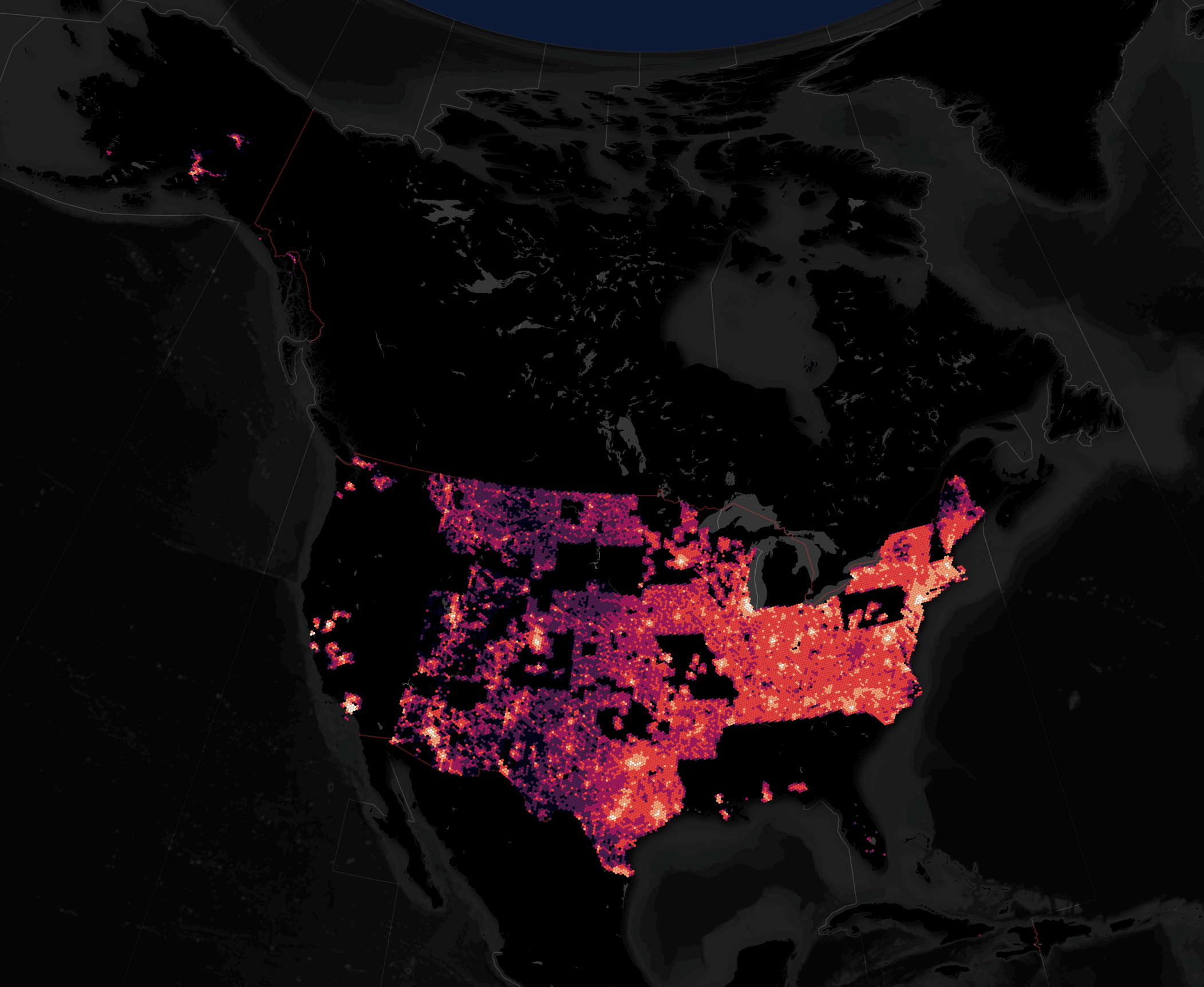
US Address Coverage
Much of the US is now represented in the US addresses dataset. There are gaps in the map but this dataset has been growing in the past few months. Hopefully it'll be filled in in a future release.
$ ~/duckdb ~/overture.duckdb
COPY (
    SELECT   h3_cell_to_boundary_wkt(
                  h3_latlng_to_cell(bbox.ymax,
                                    bbox.xmax,
                                    5))::GEOMETRY geom,
             COUNT(*) num_addresses
    FROM     READ_PARQUET('s3://overturemaps-us-west-2/release/2024-12-18.0/theme=addresses/type=address/*.parquet')
    WHERE    country = 'US'
    GROUP BY 1
) TO 'addresses.2024.12.US.gpkg'
    WITH (FORMAT GDAL,
          DRIVER 'GPKG',
          LAYER_CREATION_OPTIONS 'WRITE_BBOX=YES');
Federating Data
The one thing I'd like to see in future releases is a table that maps addresses and buildings to points of interest (POIs). This is likely a complex problem but would go a long way to both making this dataset more valuable and validating the POIs contained within Overture.
The New Bathymetry Dataset
The bathymetry theme type is made up of a single, 38 MB Parquet file containing 60,060 records.
Below is an example record. Note the sort key in the cartography dictionary. This will be helpful in rendering this dataset.
$ echo "SELECT * EXCLUDE (bbox,
                          cartography,
                          sources),
               cartography::JSON cartography,
               bbox::JSON        bbox,
               sources::JSON     sources
        FROM   READ_PARQUET('s3://overturemaps-us-west-2/release/2024-12-18.0/theme=base/type=bathymetry/*.parquet')
        LIMIT  1" \
      | ~/duckdb -json \
      | jq -S .
[
  {
    "bbox": {
      "xmax": 180.00869750976562,
      "xmin": 180.0012664794922,
      "ymax": 60.62028503417969,
      "ymin": 60.58367919921875
    },
    "cartography": {
      "max_zoom": null,
      "min_zoom": null,
      "sort_key": 12
    },
    "depth": 500,
    "geometry": "MULTIPOLYGON (((180.005302251 60.620278721, 180.003020948 60.617479661, 180.001292917 60.603416146, 180.001846188 60.59215169, 180.004680763 60.583686294, 180.006962066 60.586485354, 180.008690097 60.600548869, 180.008136825 60.611813325, 180.005302251 60.620278721)))",
    "id": "08b1749b29305fff0006d78df1434687",
    "sources": [
      {
        "confidence": null,
        "dataset": "ETOPO/GLOBathy",
        "property": "",
        "record_id": null,
        "update_time": "2024-12-11T00:00:00.000Z"
      }
    ],
    "theme": "base",
    "type": "bathymetry",
    "version": 0
  }
]
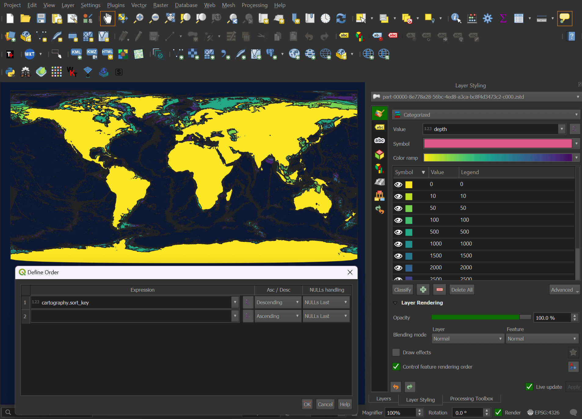
If you import the Parquet file into QGIS, under the blending mode settings for its layer, there will be a checkbox for "Control feature rendering order". In the settings, sort the "cartography.sort_key" field in descending order.
Below is a rendering of this dataset colour-coded by depth.
These are all sourced from ETOPO/GLOBathy.
$ ~/duckdb
SELECT   JSON_EXTRACT_STRING(sources::JSON->0, 'dataset') source,
         COUNT(*) num_records
FROM     READ_PARQUET('s3://overturemaps-us-west-2/release/2024-12-18.0/theme=base/type=bathymetry/*.parquet')
GROUP BY 1;
┌────────────────┬─────────────┐
│     source     │ num_records │
│    varchar     │    int64    │
├────────────────┼─────────────┤
│ ETOPO/GLOBathy │       60060 │
└────────────────┴─────────────┘
The depths only go to 3000 meters and are somewhat course in their rounding.
SELECT   depth,
         COUNT(*) num_records
FROM     READ_PARQUET('s3://overturemaps-us-west-2/release/2024-12-18.0/theme=base/type=bathymetry/*.parquet')
GROUP BY 1;
┌───────┬─────────────┐
│ depth │ num_records │
│ int32 │    int64    │
├───────┼─────────────┤
│     0 │        4285 │
│    10 │        4228 │
│    50 │        4622 │
│   100 │        3878 │
│   500 │        2748 │
│  1000 │        3308 │
│  1500 │        4722 │
│  2000 │        6750 │
│  2500 │       10309 │
│  3000 │       15210 │
├───────┴─────────────┤
│ 10 rows   2 columns │
└─────────────────────┘
The shorelines have been smoothed out. This is the Baltic Sea around Estonia's coasts overlaid on Esri's World Imagery.
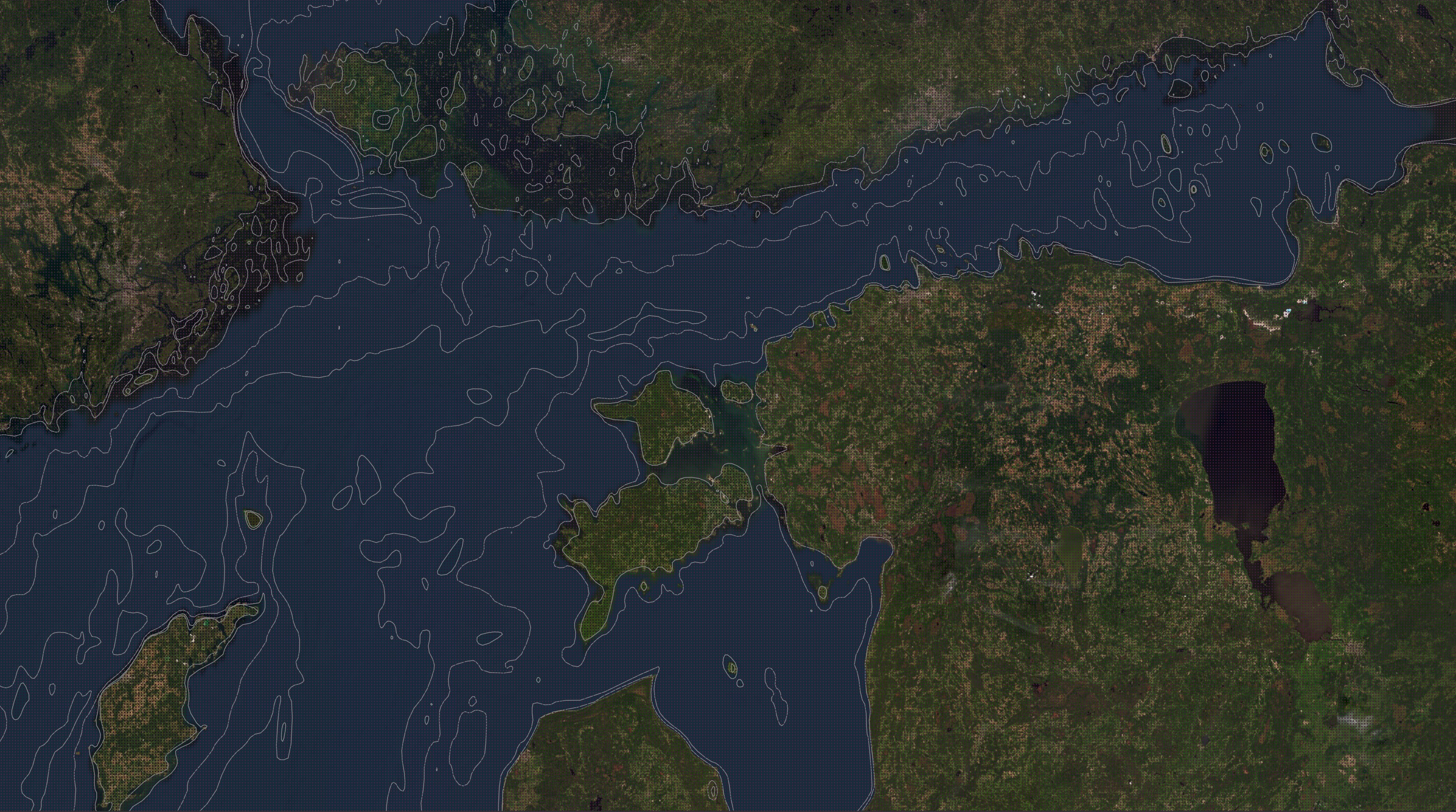
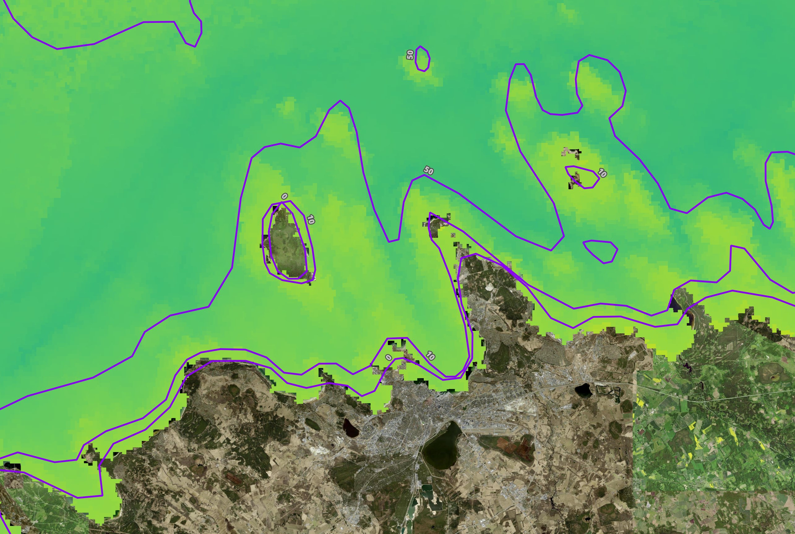
I wrote a blog post about vessel monitoring in the Baltic Sea earlier this year that used HELCOM's Baltic Sea Bathymetry Database. Overture's Bathymetry dataset is great for a convenient, global dataset in that's already in Parquet format but if you need more detailed and refined data it pays to look around.
Below is HELCOM's raster-based Bathymetry dataset with Overture's overlaid off the coast of Tallinn.
Overture's Buildings
The buildings dataset can see a lot of changes between each release. Below is the net change in buildings by country between November and this month's release.
$ ~/duckdb ~/overture.duckdb
CREATE OR REPLACE TABLE building_footprints AS
    SELECT   SPLIT(filename, '/')[5]                AS release,
             SPLIT(SPLIT(filename, '/')[8], '-')[2] AS pq_num,
             ROUND(bbox.xmin, 1)                    AS lon,
             ROUND(bbox.ymin, 1)                    AS lat,
             COUNT(*)                               AS num_buildings
    FROM     READ_PARQUET('s3://overturemaps-us-west-2/release/2024-1*/theme=buildings/type=building/*.parquet',
                            hive_partitioning=1,
                            filename=True)
    GROUP BY 1, 2, 3, 4;

CREATE OR REPLACE TABLE buildings_country_gadm AS
    SELECT   b.CONTINENT          AS continent,
             b.COUNTRY            AS country,
             a.release            AS release,
             a.pq_num             AS pq_num,
             SUM(a.num_buildings) AS num_buildings
    FROM     building_footprints a
    JOIN     gadm b ON ST_CONTAINS(b.geom,
                                   ST_POINT(a.lon, a.lat))
    GROUP BY 1, 2, 3, 4;

SELECT   country,
         SUM(num_buildings) FILTER (release='2024-12-18.0')::int128 -
         SUM(num_buildings) FILTER (release='2024-11-13.0')::int128 delta
FROM     buildings_country_gadm
GROUP BY 1
HAVING   delta != 0
ORDER BY 2 DESC;
┌──────────────────────────────────┬─────────┐
│             country              │  delta  │
│             varchar              │ int128  │
├──────────────────────────────────┼─────────┤
│ Sudan                            │ 1136940 │
│ Ethiopia                         │  714763 │
│ South Sudan                      │  528923 │
│ United States                    │  395941 │
│ Libya                            │  298453 │
│ Japan                            │  225632 │
│ Saudi Arabia                     │  179462 │
│ Chad                             │  157358 │
│ United Kingdom                   │  150885 │
│ India                            │  146677 │
│ China                            │  125931 │
│ Russia                           │  125544 │
│ Germany                          │  106389 │
│ Australia                        │   96214 │
│ Egypt                            │   91198 │
│ Italy                            │   84860 │
│ Spain                            │   81822 │
│ United Arab Emirates             │   78415 │
│ Democratic Republic of the Congo │   72817 │
│ Nigeria                          │   64946 │
│    ·                             │      ·  │
│    ·                             │      ·  │
│    ·                             │      ·  │
│ São Tomé and Príncipe            │     -11 │
│ Brunei                           │     -14 │
│ Martinique                       │     -28 │
│ Guadeloupe                       │     -33 │
│ Côte d'Ivoire                    │     -87 │
│ Trinidad and Tobago              │    -109 │
│ Angola                           │    -170 │
│ Namibia                          │    -198 │
│ Suriname                         │    -319 │
│ Réunion                          │    -501 │
│ Eritrea                          │    -547 │
│ French Guiana                    │    -838 │
│ Burkina Faso                     │    -911 │
│ Puerto Rico                      │    -932 │
│ Guatemala                        │    -935 │
│ Paraguay                         │    -984 │
│ Sri Lanka                        │   -1073 │
│ Zimbabwe                         │   -1467 │
│ Swaziland                        │   -1506 │
│ El Salvador                      │   -7592 │
├──────────────────────────────────┴─────────┤
│ 222 rows (40 shown)              2 columns │
└────────────────────────────────────────────┘
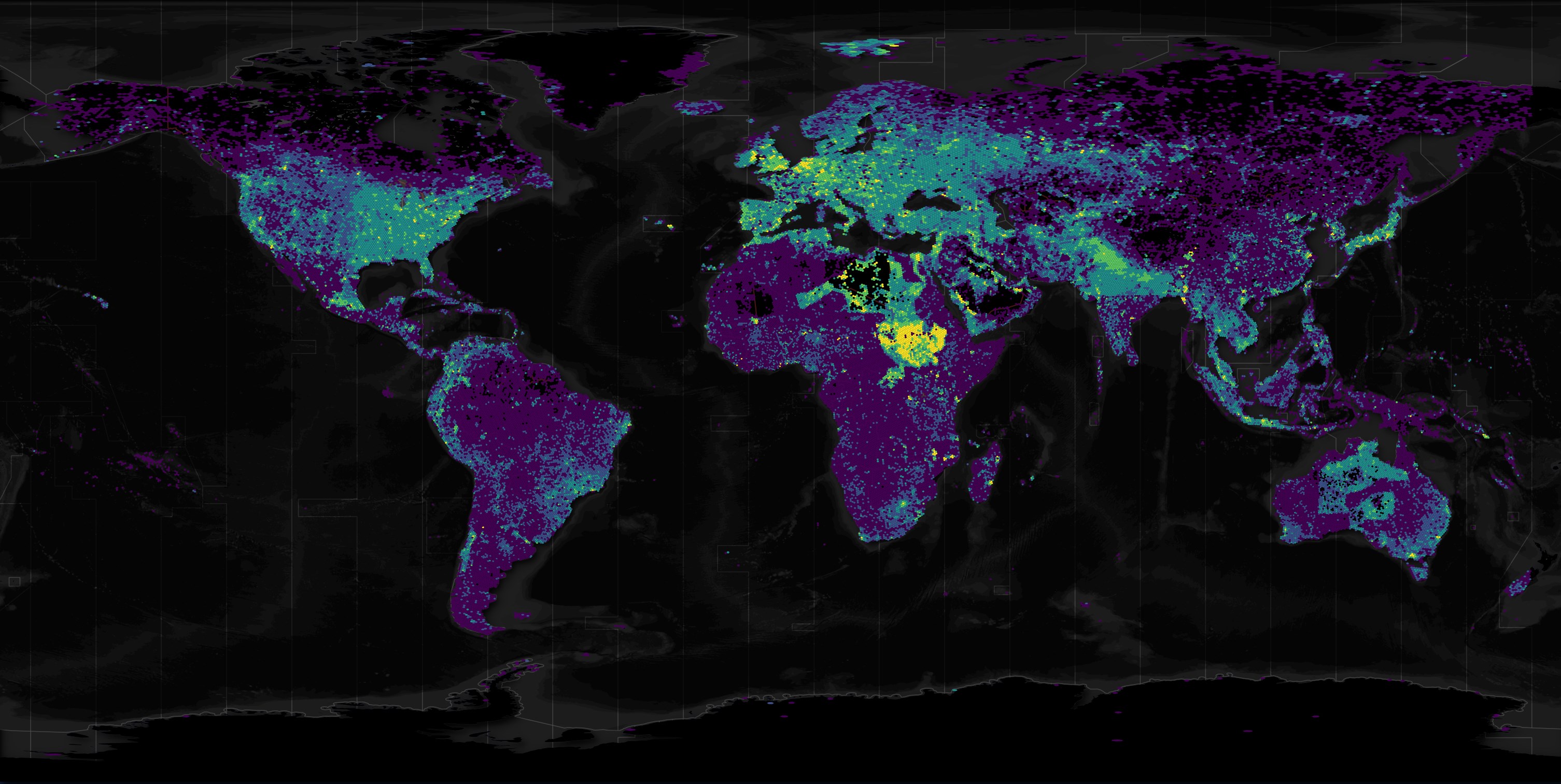
Below I'll put together a heatmap of the changes seen this month.
CREATE OR REPLACE TABLE h3_4_stats AS
    SELECT   H3_LATLNG_TO_CELL(lat, lon, 4) as h3_4,
             SUM(num_buildings) FILTER (release='2024-12-18.0')::int32 -
             SUM(num_buildings) FILTER (release='2024-11-13.0')::int32 delta
    FROM     building_footprints
    WHERE    lon < 172
    AND      lon > -172
    GROUP BY 1;

COPY (
    SELECT H3_CELL_TO_BOUNDARY_WKT(h3_4)::geometry geom,
           delta
    FROM   h3_4_stats
) TO 'building_changes.h3_4.gpkg'
    WITH (FORMAT GDAL,
          DRIVER 'GPKG',
          LAYER_CREATION_OPTIONS 'WRITE_BBOX=YES');
The brightest areas saw the greatest net increase in building footprints over the past month while the darkest saw either no change or a slight net decrease.
Overture's Roads
Road data is broken up into connector and segment theme types. Measuring by disk usage in GB, both datasets have been fairly stable in the past few months.
$ ~/duckdb ~/overture.duckdb
WITH a AS (
    SELECT   theme_type,
             release,
             ROUND(SUM(Size) / 1024 ** 3)::INT sum_size
    FROM     s3
    WHERE    theme = 'transportation'
    GROUP BY 1, 2
)
PIVOT    a
ON       theme_type
USING    SUM(sum_size)
ORDER BY release;
┌────────────────────┬───────────┬─────────┐
│      release       │ connector │ segment │
│      varchar       │  int128   │ int128  │
├────────────────────┼───────────┼─────────┤
│ 2023-07-26-alpha.0 │        20 │      62 │
│ 2023-10-19-alpha.0 │        20 │      61 │
│ 2023-11-14-alpha.0 │        18 │      58 │
│ 2023-12-14-alpha.0 │        17 │      46 │
│ 2024-01-17-alpha.0 │        17 │      46 │
│ 2024-02-15-alpha.0 │        17 │      47 │
│ 2024-03-12-alpha.0 │        18 │      48 │
│ 2024-04-16-beta.0  │        12 │      44 │
│ 2024-05-16-beta.0  │        14 │      44 │
│ 2024-06-13-beta.0  │        13 │      45 │
│ 2024-06-13-beta.1  │        13 │      45 │
│ 2024-07-22.0       │        13 │      46 │
│ 2024-08-20.0       │        13 │      52 │
│ 2024-09-18.0       │        13 │      55 │
│ 2024-10-23.0       │        13 │      49 │
│ 2024-11-13.0       │        13 │      50 │
│ 2024-12-18.0       │        13 │      50 │
├────────────────────┴───────────┴─────────┤
│ 17 rows                        3 columns │
└──────────────────────────────────────────┘
Below is the net change by country between October and this month's release.
CREATE OR REPLACE TABLE roads AS
    SELECT   SPLIT(filename, '/')[5] AS release,
             ROUND(bbox.xmin, 1) AS lon,
             ROUND(bbox.ymin, 1) AS lat,
             COUNT(*) AS num_roads
    FROM     READ_PARQUET('s3://overturemaps-us-west-2/release/2024-1*/theme=transportation/type=segment/*.parquet',
                          hive_partitioning=1,
                          filename=True)
    GROUP BY 1, 2, 3;

CREATE OR REPLACE TABLE roads_country AS
    SELECT   b.COUNTRY AS country,
             a.release AS release,
             SUM(a.num_roads) AS num_roads
    FROM     roads a
    JOIN     gadm b ON ST_CONTAINS(b.geom,
                                   ST_POINT(a.lon, a.lat))
    GROUP BY 1, 2;

SELECT   country,
         SUM(num_roads) FILTER (release='2024-12-18.0')::int128 -
         SUM(num_roads) FILTER (release='2024-10-23.0')::int128 delta
FROM     roads_country
GROUP BY 1
HAVING   delta != 0
ORDER BY 2 DESC;
┌──────────────────────────────────┬────────┐
│             country              │ delta  │
│             varchar              │ int128 │
├──────────────────────────────────┼────────┤
│ United States                    │ 486493 │
│ India                            │ 287099 │
│ Myanmar                          │ 217286 │
│ China                            │ 207824 │
│ France                           │ 122398 │
│ Germany                          │  77386 │
│ Spain                            │  72846 │
│ Poland                           │  71973 │
│ Guatemala                        │  68542 │
│ Canada                           │  63234 │
│ United Kingdom                   │  60958 │
│ Japan                            │  56353 │
│ Brazil                           │  56134 │
│ Italy                            │  53793 │
│ Russia                           │  50848 │
│ Pakistan                         │  46721 │
│ Australia                        │  38043 │
│ Uzbekistan                       │  32904 │
│ South Korea                      │  31099 │
│ Iran                             │  30110 │
│  ·                               │      · │
│  ·                               │      · │
│  ·                               │      · │
│ Jersey                           │     12 │
│ Cabo Verde                       │     12 │
│ Seychelles                       │     10 │
│ Solomon Islands                  │      7 │
│ Cayman Islands                   │      5 │
│ Saint Pierre and Miquelon        │      5 │
│ Niue                             │      5 │
│ Samoa                            │      5 │
│ Antarctica                       │      5 │
│ Antigua and Barbuda              │      4 │
│ Falkland Islands                 │      3 │
│ South Georgia and the South Sand │      2 │
│ Dominica                         │      2 │
│ São Tomé and Príncipe            │      2 │
│ Virgin Islands, U.S.             │      1 │
│ Faroe Islands                    │      1 │
│ Christmas Island                 │      1 │
│ British Indian Ocean Territory   │     -1 │
│ Saint Kitts and Nevis            │     -6 │
│ Burundi                          │   -230 │
├──────────────────────────────────┴────────┤
│ 219 rows (40 shown)             2 columns │
└───────────────────────────────────────────┘
Extracting a City's Buildings
Up until last week, if I wanted to extract a city-sized area from the buildings dataset, I'd first find out which Parquet files contained data for the country that city is in. Below are the Parquet file numbers for Iran's data in the November release.
SELECT   pq_num,
         SUM(num_buildings)
FROM     buildings_country_gadm
WHERE    release = '2024-11-13.0'
AND      country = 'Iran'
GROUP BY 1
ORDER BY 2 DESC;
┌─────────┬────────────────────┐
│ pq_num  │ sum(num_buildings) │
│ varchar │       int128       │
├─────────┼────────────────────┤
│ 00129   │            6494017 │
│ 00128   │            3928784 │
│ 00127   │             572505 │
│ 00130   │             292240 │
│ 00110   │             261544 │
│ 00111   │              18776 │
└─────────┴────────────────────┘
I'd then download those Parquet files first and then extract out any buildings within a bounding box for the city of interest. Working with Parquet files on a local SSD was often 5x faster than working with them remotely on S3.
Below is the code to extract Tehran's building footprints from the November release.
COPY (
    SELECT a.* EXCLUDE (names,
                        bbox,
                        sources,
                        geometry),
           JSON(a.names)                        AS names,
           JSON(a.bbox)                         AS bbox,
           JSON(a.sources)                      AS sources,
           ST_ASWKB(a.geometry) AS geom
    FROM   READ_PARQUET([
            'part-00129*.parquet',
            'part-00128*.parquet',
            'part-00127*.parquet',
            'part-00130*.parquet',
            'part-00110*.parquet',
            'part-00111*.parquet',
        ]) a
    WHERE  bbox.xmin > 50.7993
    AND    bbox.xmax < 51.8616
    AND    bbox.ymin > 35.3870
    AND    bbox.ymax < 36.0667
ORDER BY   HILBERT_ENCODE([ST_Y(ST_CENTROID(a.geometry)),
                           ST_X(ST_CENTROID(a.geometry))]::double[2])
) TO 'iran.2024.11.buildings.pq' (
    FORMAT            'PARQUET',
    CODEC             'ZSTD',
    COMPRESSION_LEVEL 22,
    ROW_GROUP_SIZE    15000);
The result would be a file that was produced from gigabytes of source data but ultimately only contained tens of megabytes of data of interest.
$ python ~/pqview/main.py \
    sizes \
    iran.2024.11.buildings.pq
 70.2 MB geom
 16.4 MB bbox
  9.8 MB sources
  7.6 MB id
147.0 kB names
 37.9 kB subtype
 36.3 kB class
 18.8 kB height
 11.2 kB num_floors
  4.9 kB level
  3.8 kB roof_shape
  3.4 kB roof_color
  3.0 kB has_parts
  3.0 kB version
  2.9 kB is_underground
  2.7 kB facade_color
  2.5 kB facade_material
  2.4 kB num_floors_underground
  2.4 kB roof_orientation
  2.4 kB min_floor
  2.3 kB min_height
  2.3 kB roof_height
  2.3 kB roof_material
  2.2 kB roof_direction
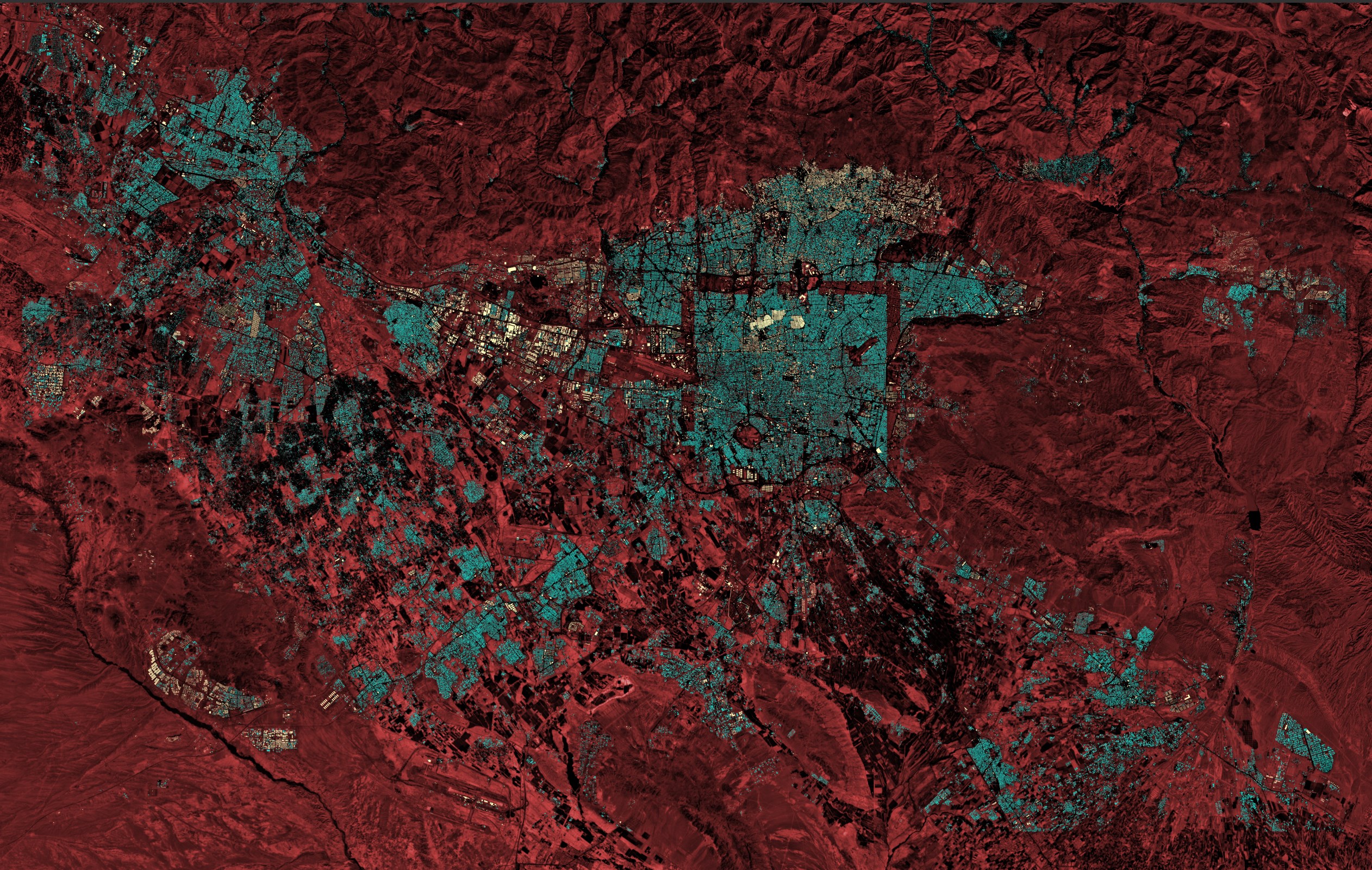
This is the above Parquet file rendered in QGIS. The basemap is Esri's World Imagery basemap. It has been tinted red to contrast it with the colour-coded building footprints covering it.
But last week, I found a faster and simpler way to extract city-level data from Overture.
QGIS Integration
Chris Holmes, who is a Fellow and Vice President at Planet Labs, recently published a QGIS GeoParquet Downloader plugin. This plugin will take the bounding box of your QGIS workspace and only download the data for that area. Many data sources are supported including Overture, Source Cooperative and Hugging Face.
Before installing the plugin, go to the Plugins Menu in QGIS and click "Python Console". Then type:
import pip; pip.main(['install', '--upgrade', 'duckdb'])
Next, click on the Plugins Menu and then "Manage and Install Plugins".
Select "All" from the top left and search for "GeoParquet Downloader". Click the "Install Plugin" button on the bottom right of the UI.
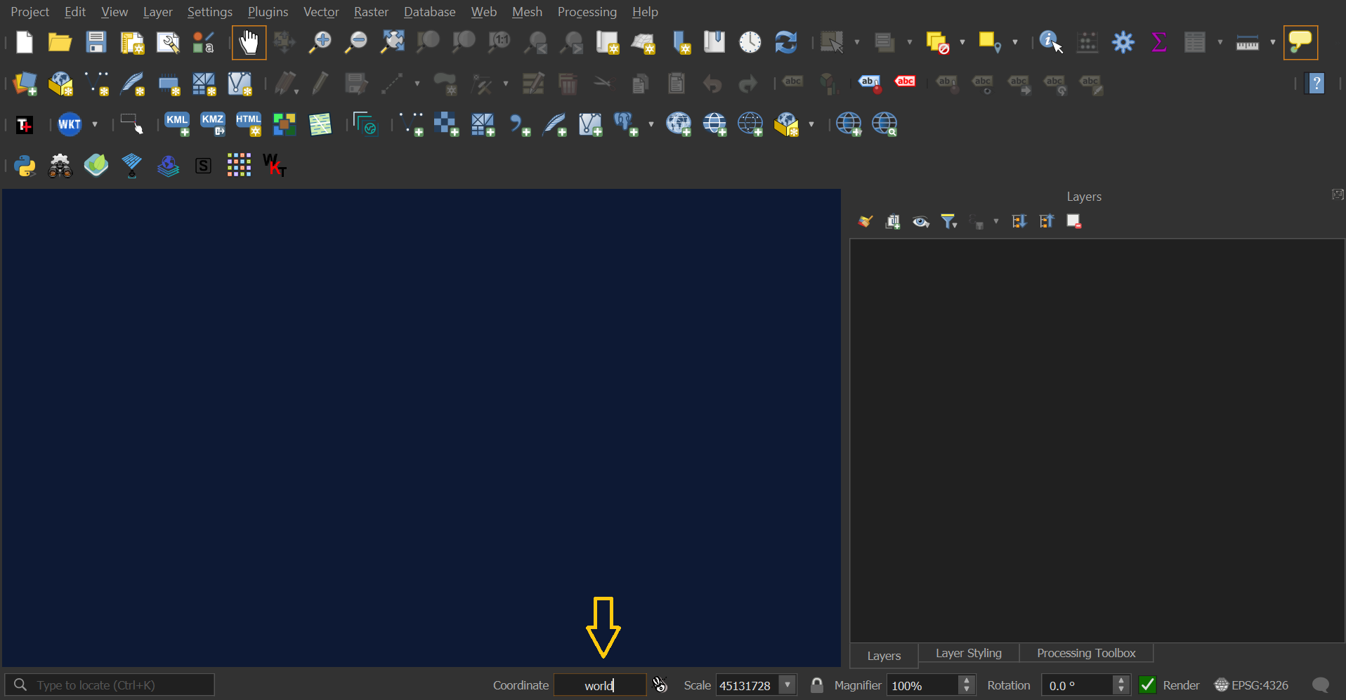
Then, in the middle of the bottom toolbar, type "world" into the coordinates text box and hit enter. A vector map of the world should appear.
Zoom into a city of interest somewhere in the world and then click the "Download Overture Maps Data" button in one of the top toolbars. The button's position can vary depending on how you've configured QGIS' layout.
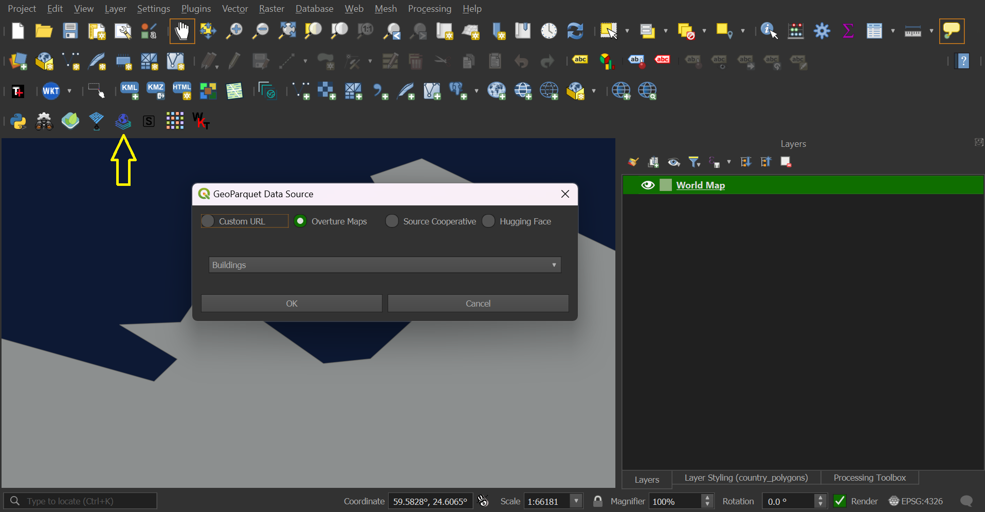
Select "Buildings" from the UI that pops up and save the results to a GeoParquet file. The data should appear in the QGIS workspace shortly after it has been downloaded into that GeoParquet file.
Overture's buildings all have numerous metadata fields that can be used to aid visualisation and analysis.

The GeoParquet file for the above scene is less than 8 MB in size. When uncompressed and in JSON format the data is over 57 MB in size.
$ echo "FROM 'geoparquet_download_20241211_113210.parquet'" \
    | ~/duckdb -json \
    | wc -c
60200446
Below is an example record.
$ echo "FROM  'geoparquet_download_20241211_113210.parquet'
        WHERE roof_color    IS NOT NULL
        AND   roof_material IS NOT NULL
        LIMIT 1" \
    | ~/duckdb -json \
    | jq -S .
[
  {
    "bbox": "{'xmin': 24.72516, 'xmax': 24.725378, 'ymin': 59.430557, 'ymax': 59.430717}",
    "class": "apartments",
    "facade_color": null,
    "facade_material": null,
    "geometry": "POLYGON ((24.725212 59.430564, 24.725378 59.43058, 24.7253552 59.430648, 24.725332 59.430717, 24.725164 59.430702, 24.725212 59.430564))",
    "has_parts": false,
    "height": null,
    "id": "08b089b1a6082fff0200faf2a07a0508",
    "is_underground": false,
    "level": null,
    "min_floor": null,
    "min_height": null,
    "names": null,
    "num_floors": 2,
    "num_floors_underground": null,
    "roof_color": "#C0C0C0",
    "roof_direction": null,
    "roof_height": null,
    "roof_material": "metal",
    "roof_orientation": null,
    "roof_shape": "hipped",
    "sources": "[{'property': , 'dataset': OpenStreetMap, 'record_id': w26897528@6, 'update_time': 2023-07-12T17:34:53.000Z, 'confidence': NULL}]",
    "subtype": "residential",
    "theme": "buildings",
    "type": "building",
    "version": 0
  }
]
The Map Explorer
Overture's Map Explorer was released a few months ago. It's intended as an x-ray viewer of their datasets meaning it helps inspect individual records in a 2D and 3D map interface.
Overture hosts the map's data in 370+ GB worth of PMTiles on AWS Cloudfront. The viewer selectively downloads data within the field of view from these files, saving a huge amount of bandwidth and loading areas of interest in real-time as you zoom and pan the map.
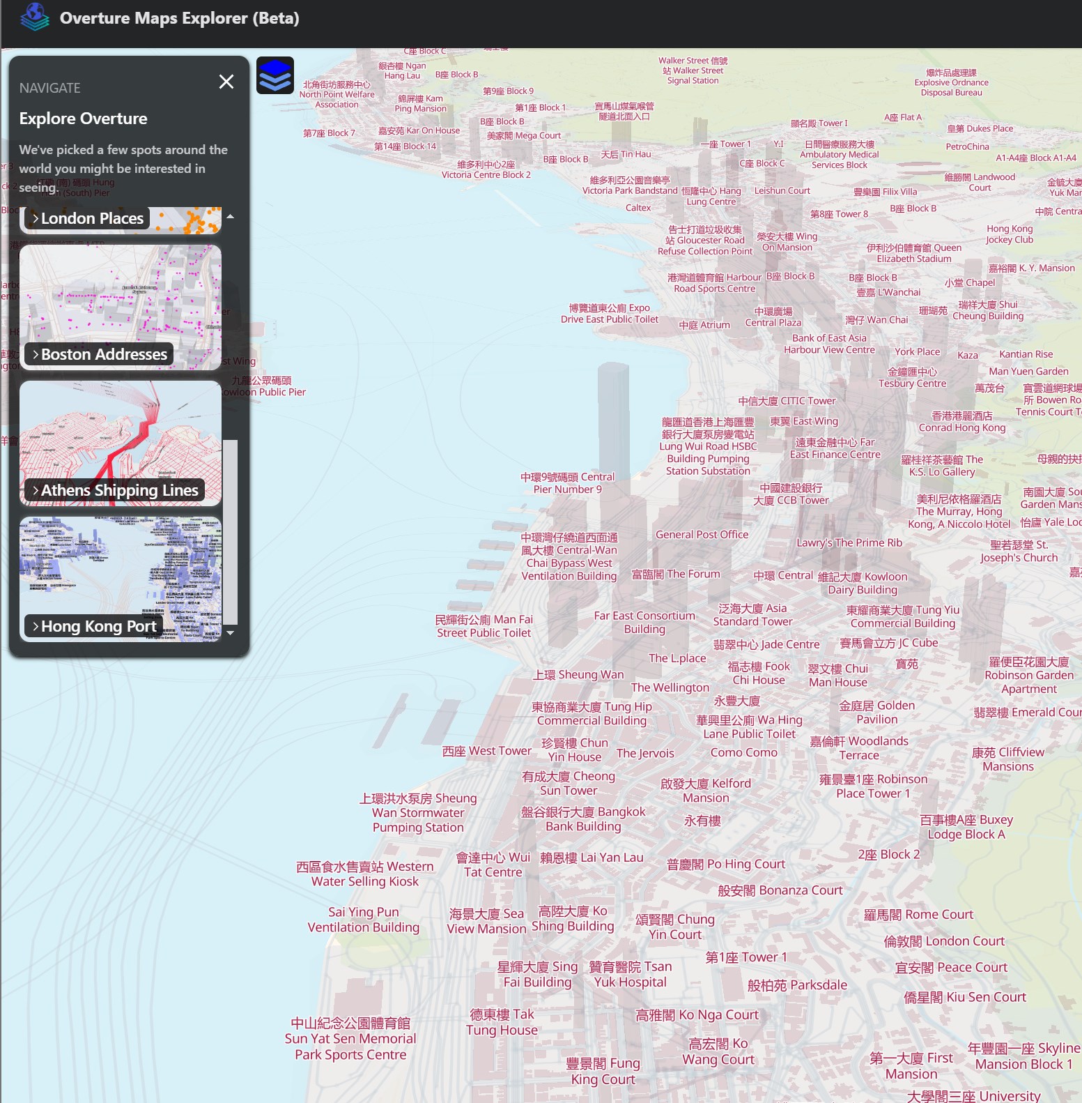
They've recently added bookmarks to the UI that introduce places and map functionality of interest. Included in these are 3D buildings. Below is a screenshot of Hong Kong.
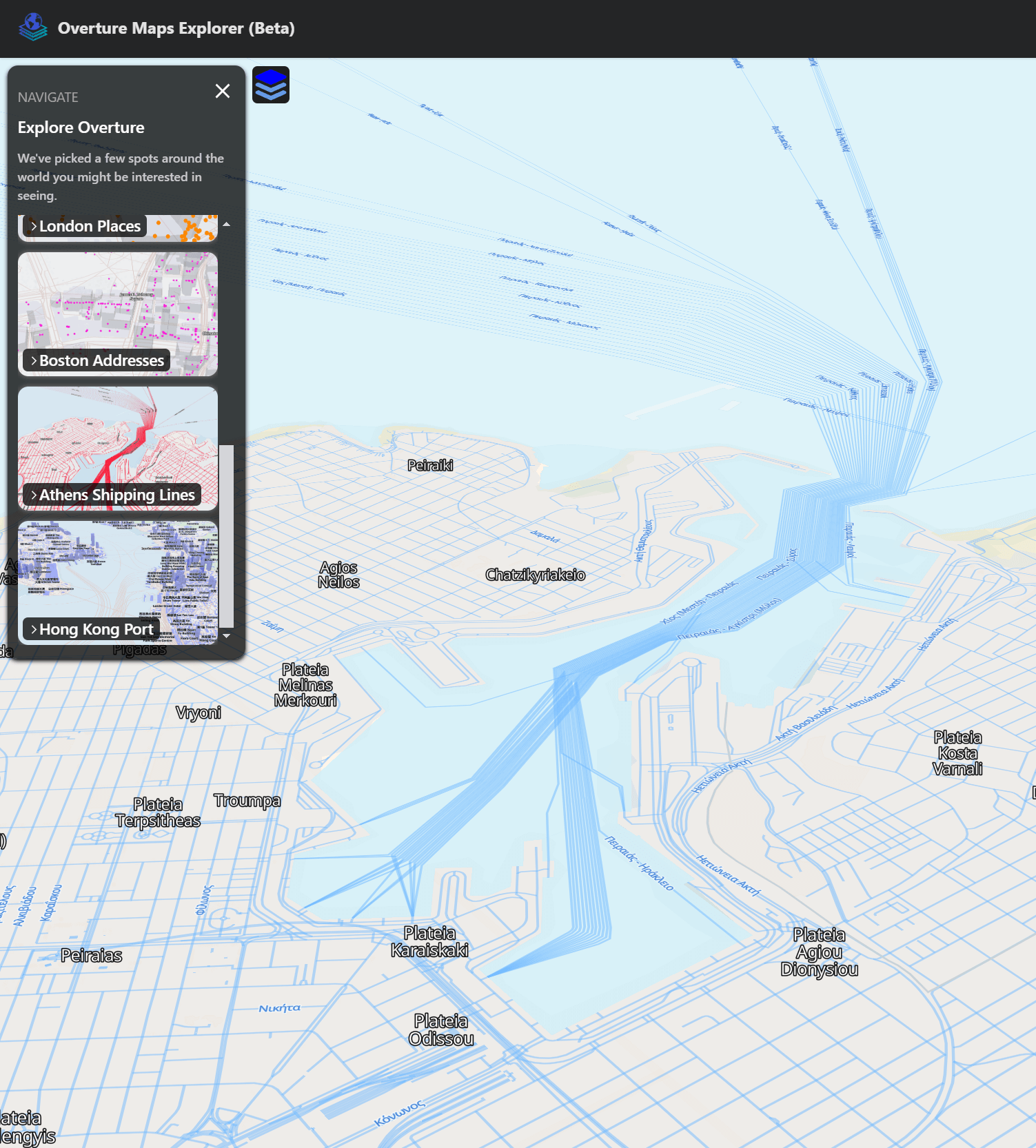
They also have a bookmark for the shipping lanes leaving the Port of Piraeus just outside of Athens.
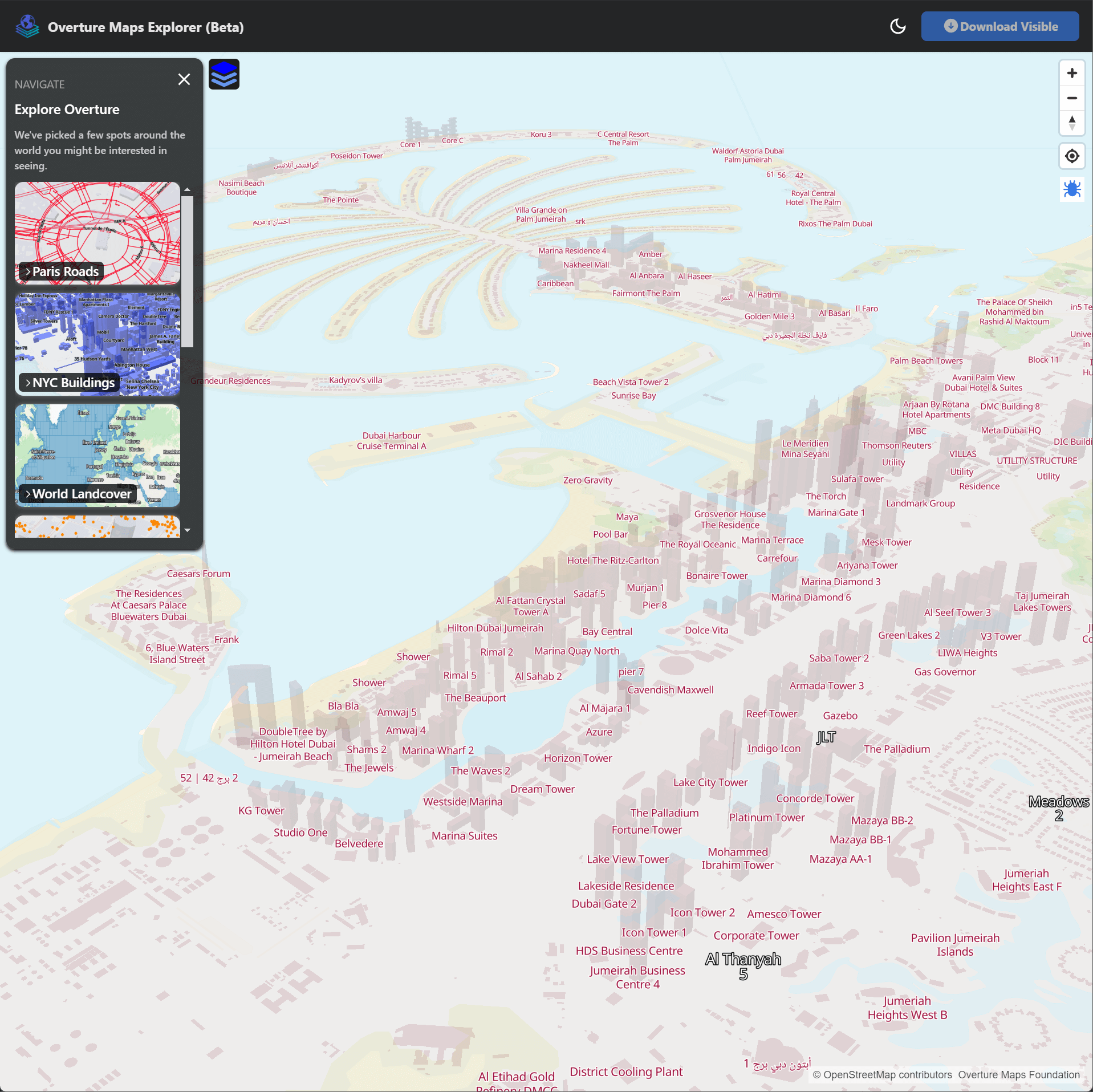
Below is Dubai's Jumeirah Beach Residence (JBR) area with the Palm Jumeirah archipelago in the background.
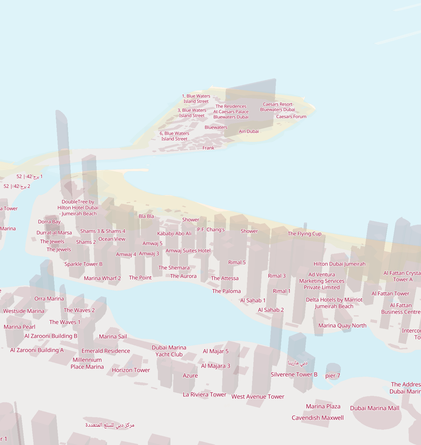
Not all notable structures have representative 3D models. For example, Ain Dubai, the world's highest observation wheel appears as a thin rectangle.
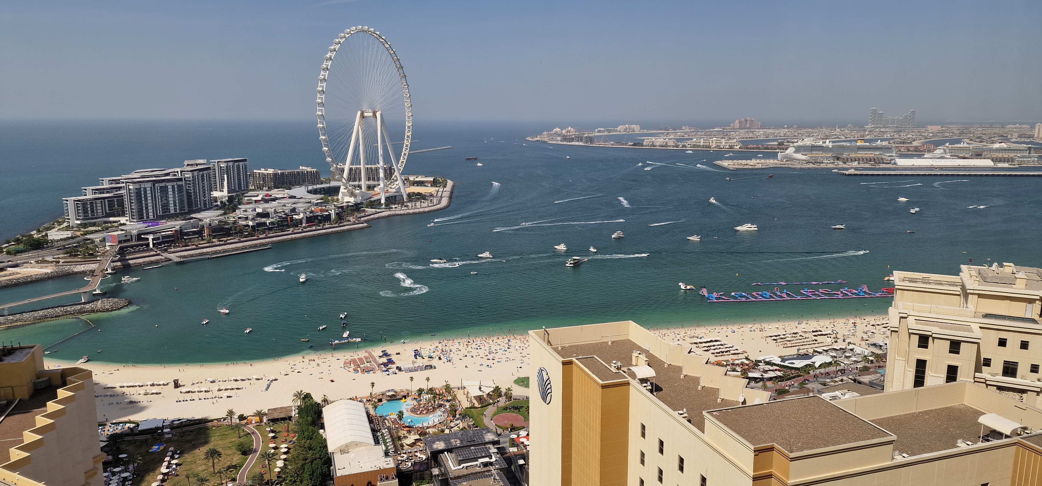
This is the Ain Dubai in real life.
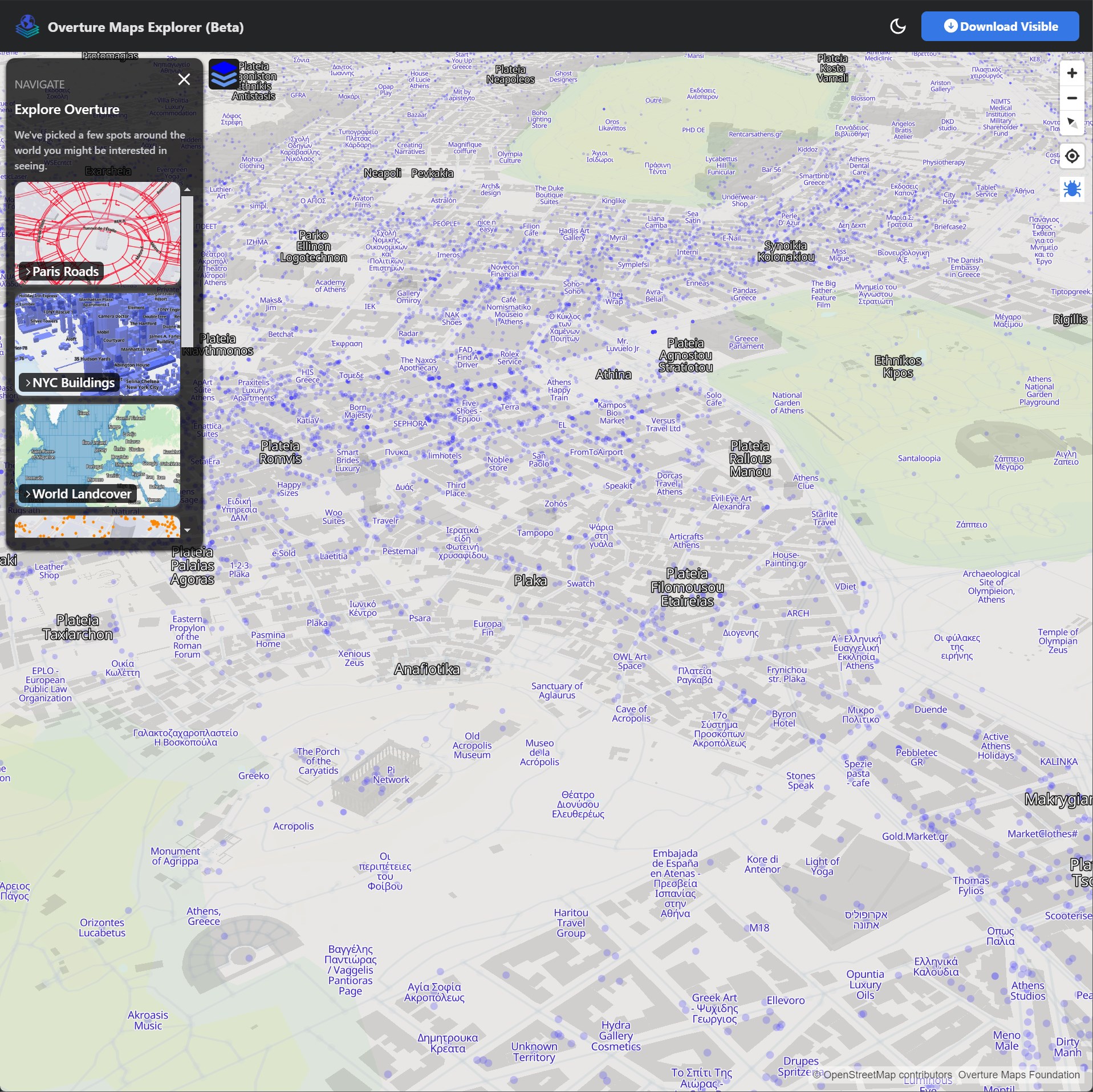
It would be nice to see support for Digital Elevation Models (DEMs) added to this viewer. Cities like Athens can be difficult to navigate around without any topography to aid orientation.
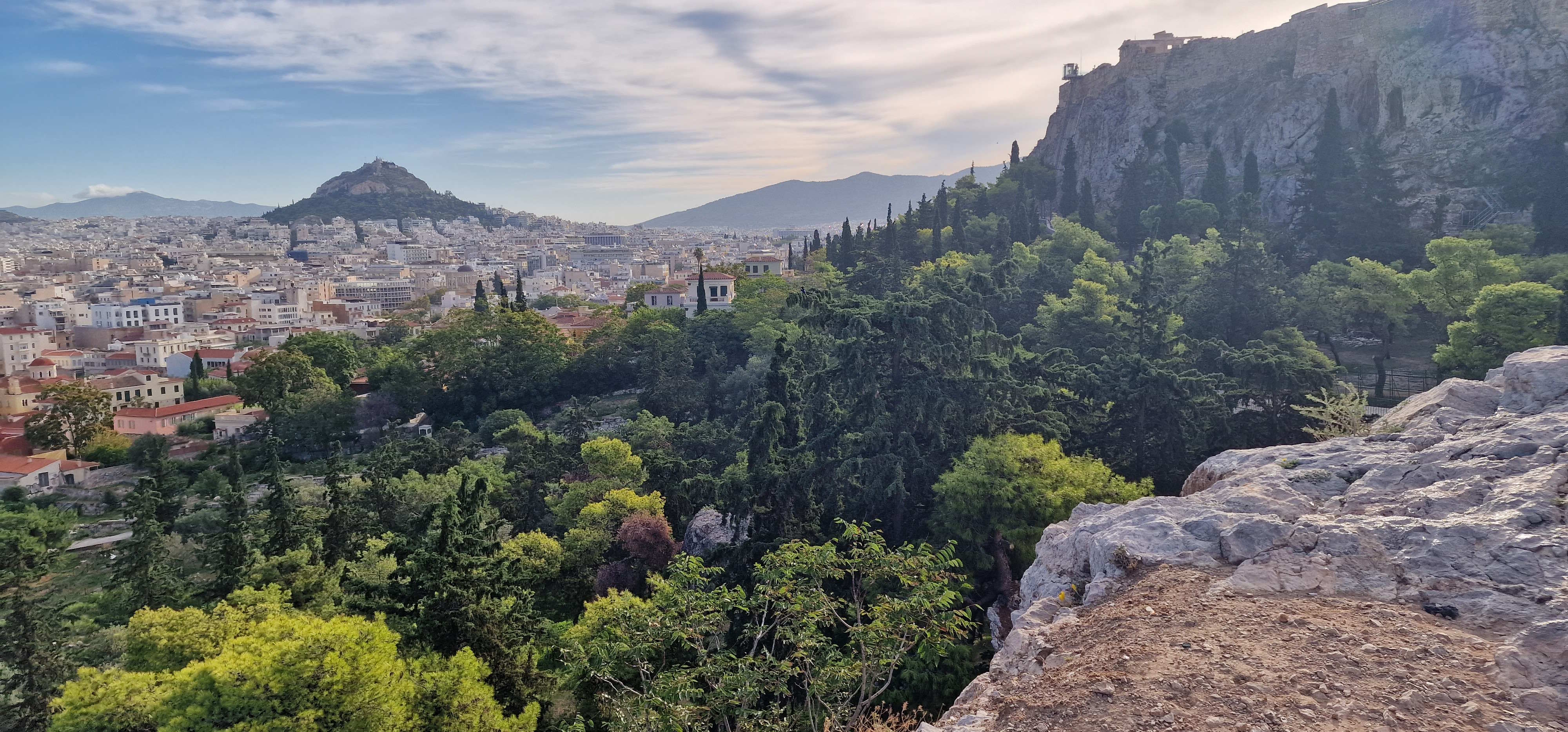
Below is the same area in real life. The topography tells the story of the city's layout.
Qiusheng Wu's Python-based leafmap project supports both 3D Terrain and 3D PMTiles so at least one web-based, open source solution does exist.
Extracting 3D Building Parts
Selecting any 3D building in the Explorer will bring up its properties.
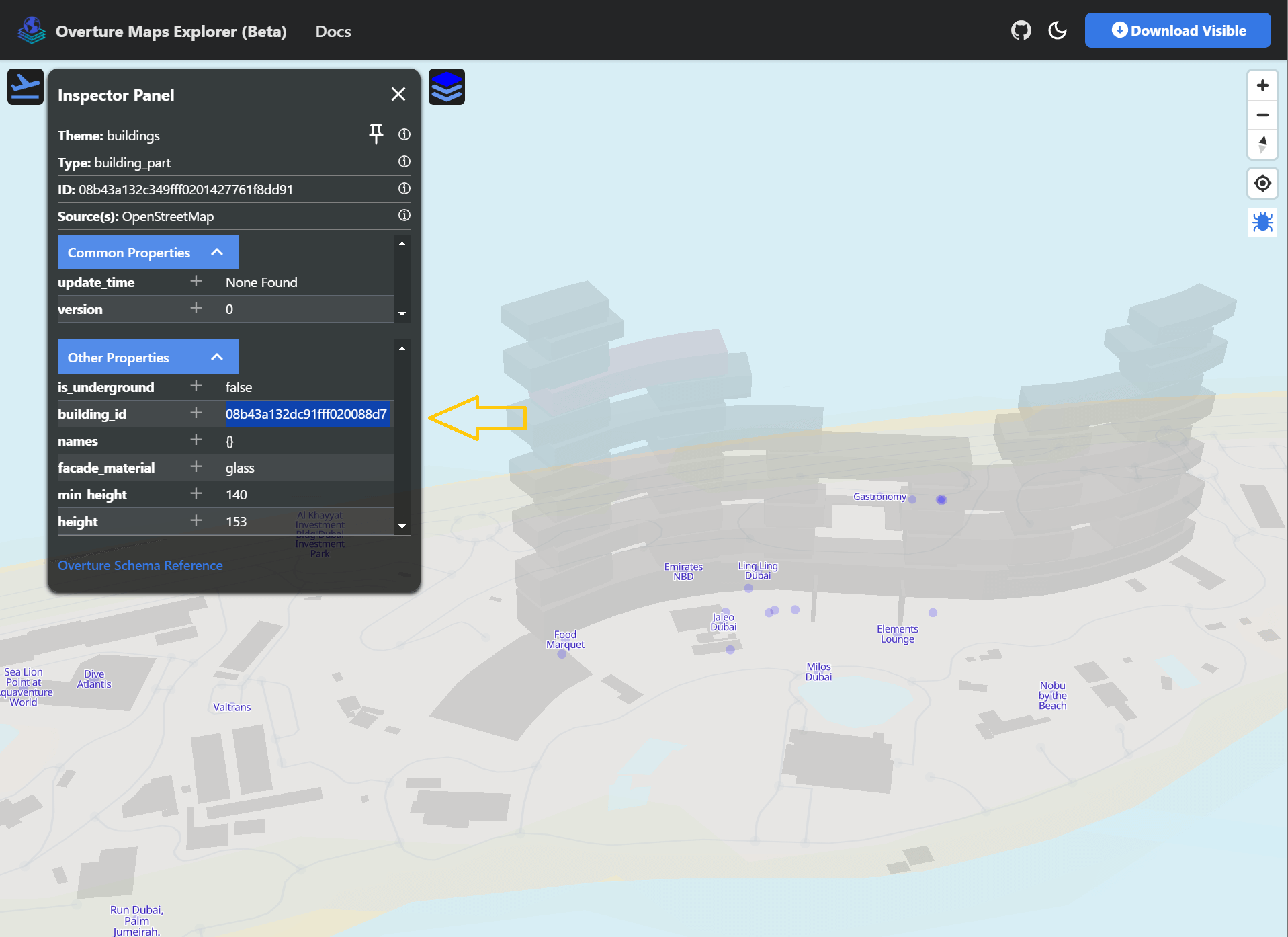
The building_id field (not to be confused with the id field) can be used to search the building_part dataset.
$ echo "FROM  READ_PARQUET('s3://overturemaps-us-west-2/release/2024-12-18.0/theme=buildings/type=building_part/*.parquet',
                           hive_partitioning=1,
                           filename=True)
        WHERE building_id = '08b43a132dc91fff020088d7020f24e2'" \
    | ~/duckdb -json \
    | jq -S 'del(..|nulls)' \
    > cloud_22.json
The above returned 31 records, each with its own properties and polygons.
$ jq length cloud_22.json # 31
Below is an example record.
$ jq -S '.[0]' cloud_22.json
{
  "bbox": "{'xmin': 55.125946, 'xmax': 55.126446, 'ymin': 25.137445, 'ymax': 25.137896}",
  "building_id": "08b43a132dc91fff020088d7020f24e2",
  "facade_material": "glass",
  "filename": "s3://overturemaps-us-west-2/release/2024-12-18.0/theme=buildings/type=building_part/part-00000-00ec12bf-9729-48e6-b5e9-4ecfd7a91363-c000.zstd.parquet",
  "geometry": "POLYGON ((55.1259462 25.1375893, 55.1260403 25.1375121, 55.1261211 25.1374458, 55.1262212 25.1375423, 55.1263344 25.1376442, 55.1264449 25.1377377, 55.1262972 25.1378926, 55.1261991 25.1378181, 55.1260941 25.1377271, 55.1259462 25.1375893))",
  "height": 137.0,
  "id": "08b43a132c348fff02013812c88f362f",
  "is_underground": false,
  "min_height": 124.0,
  "names": "{'primary': NULL, 'common': NULL, 'rules': NULL}",
  "sources": "[{'property': , 'dataset': OpenStreetMap, 'record_id': w964652257, 'update_time': 2024-05-27T11:05:56.000Z, 'confidence': NULL}]",
  "theme": "buildings",
  "type": "building_part",
  "version": 0
}
Below are a few properties for each of the 31 polygons.
$ jq -c '.[]|[.min_height,.height,.facade_material]' cloud_22.json
[124.0,137.0,"glass"]
[184.0,193.0,"glass"]
[24.0,41.0,"glass"]
[60.0,73.0,"glass"]
[92.0,105.0,"glass"]
[156.0,169.0,"glass"]
[null,189.0,"glass"]
[172.0,181.0,"glass"]
[null,22.0,null]
[76.0,89.0,"glass"]
[140.0,153.0,"glass"]
[44.0,57.0,"glass"]
[109.0,121.0,"glass"]
[null,145.0,"glass"]
[124.0,137.0,"glass"]
[24.0,41.0,"glass"]
[60.0,73.0,"glass"]
[92.0,105.0,"glass"]
[44.0,57.0,"glass"]
[90.0,92.0,null]
[null,20.0,null]
[76.0,90.0,"glass"]
[24.0,41.0,"glass"]
[60.0,73.0,"glass"]
[92.0,105.0,"glass"]
[76.0,89.0,"glass"]
[44.0,57.0,"glass"]
[null,21.0,"glass"]
[140.0,149.0,"glass"]
[null,157.0,"glass"]
[92.0,105.0,"glass"]