Since May, Overture Maps has been publishing a global, open dataset of land cover. This data is in vector form and distinguishes between ten types of land cover: barren, crop, forest, grass, mangrove, moss, shrub, snow, urban and wetlands.
The classifications were produced from imagery provided by the European Space Agency’s 2020 WorldCover dataset. The source imagery has a resolution of 10m and was captured by the Sentinel-1 and Sentinel-2 satellites between 2020 and 2021.
Below is a rendering of Overture's data for Tallinn, Estonia.

The vector data is made up of 117,644,836 records and shipped as 84, geospatially-sorted, ZStandard-compressed Parquet files. This is the gold standard for sharing large GIS data. However, despite that, opening individual countries or regions locally can be challenging.
In this post, I'll walk through identifying the regions, countries and continents of Overture's land cover dataset and extract Australia's Land Cover records.
My Workstation
I'm using a 6 GHz Intel Core i9-14900K CPU. It has 8 performance cores and 16 efficiency cores with a total of 32 threads and 32 MB of L2 cache. It has a liquid cooler attached and is housed in a spacious, full-sized, Cooler Master HAF 700 computer case. I've come across videos on YouTube where people have managed to overclock the i9-14900KF to 9.1 GHz.
The system has 96 GB of DDR5 RAM clocked at 6,000 MT/s and a 5th-generation, Crucial T700 4 TB NVMe M.2 SSD which can read at speeds up to 12,400 MB/s. There is a heatsink on the SSD to help keep its temperature down. This is my system's C drive.
The system is powered by a 1,200-watt, fully modular, Corsair Power Supply and is sat on an ASRock Z790 Pro RS Motherboard.
I'm running Ubuntu 22 LTS via Microsoft's Ubuntu for Windows on Windows 11 Pro. In case you're wondering why I don't run a Linux-based desktop as my primary work environment, I'm still using an Nvidia GTX 1080 GPU which has better driver support on Windows and I use ArcGIS Pro from time to time which only supports Windows natively.
Installing Prerequisites
I'll be using a few other tools to help download and analyse the data in this post.
$ sudo apt update
$ sudo apt install \
    aws-cli \
    jq
I'll also use DuckDB, along with its H3, JSON, Parquet and Spatial extensions.
$ cd ~
$ wget -c https://github.com/duckdb/duckdb/releases/download/v1.1.1/duckdb_cli-linux-amd64.zip
$ unzip -j duckdb_cli-linux-amd64.zip
$ chmod +x duckdb
$ ~/duckdb
INSTALL h3 FROM community;
INSTALL json;
INSTALL parquet;
INSTALL spatial;
I'll set up DuckDB to load every installed extension each time it launches.
$ vi ~/.duckdbrc
.timer on
.width 180
LOAD h3;
LOAD json;
LOAD parquet;
LOAD spatial;
The maps in this post were rendered with QGIS version 3.38.0. QGIS is a desktop application that runs on Windows, macOS and Linux. The application has grown in popularity in recent years and has ~15M application launches from users around the world each month.
I used QGIS' Tile+ plugin to add geospatial context with CARTO's Basemaps to the maps.
Downloading Overture's Data
Overture tends to publish a new dataset in the middle of each month. The following will list each publication they've made.
$ aws s3 --no-sign-request ls s3://overturemaps-us-west-2/release/
PRE 2023-04-02-alpha/
PRE 2023-07-26-alpha.0/
PRE 2023-10-19-alpha.0/
PRE 2023-11-14-alpha.0/
PRE 2023-12-14-alpha.0/
PRE 2024-01-17-alpha.0/
PRE 2024-02-15-alpha.0/
PRE 2024-03-12-alpha.0/
PRE 2024-04-16-beta.0/
PRE 2024-05-16-beta.0/
PRE 2024-06-13-beta.0/
PRE 2024-06-13-beta.1/
PRE 2024-07-22.0/
PRE 2024-08-20.0/
PRE 2024-09-18.0/
I'll download the 84 GB of parquet data for their land cover dataset from September's release.
$ aws s3 --no-sign-request sync \
    s3://overturemaps-us-west-2/release/2024-09-18.0/theme=base/type=land_cover/ \
    ~/land_cover
It is possible to work with Overture's Parquet files on S3 rather than storing them locally but I found querying their data on an SATA-backed SSD was ~5x faster than off of S3 on my 500 Mbps broadband connection.
GeoFabrik's OSM Partitions
GeoFabrik publishes a GeoJSON file that shows all of the spatial partitions they use for their OpenStreetMap (OSM) releases. I'll use these partitions to help cluster Overture's records by region.
$ wget -O ~/geofabrik.geojson \
    https://download.geofabrik.de/index-v1.json
Below is an example record. I've excluded the geometry field for readability.
$ jq -S '.features[0]' ~/geofabrik.geojson \
    | jq 'del(.geometry)'
{
  "properties": {
    "id": "afghanistan",
    "iso3166-1:alpha2": [
      "AF"
    ],
    "name": "Afghanistan",
    "parent": "asia",
    "urls": {
      "bz2": "https://download.geofabrik.de/asia/afghanistan-latest.osm.bz2",
      "history": "https://osm-internal.download.geofabrik.de/asia/afghanistan-internal.osh.pbf",
      "pbf": "https://download.geofabrik.de/asia/afghanistan-latest.osm.pbf",
      "pbf-internal": "https://osm-internal.download.geofabrik.de/asia/afghanistan-latest-internal.osm.pbf",
      "shp": "https://download.geofabrik.de/asia/afghanistan-latest-free.shp.zip",
      "taginfo": "https://taginfo.geofabrik.de/asia:afghanistan",
      "updates": "https://download.geofabrik.de/asia/afghanistan-updates"
    }
  },
  "type": "Feature"
}
These partitions cover anywhere with a landmass on Earth.
I'll import GeoFabrik's spatial partitions into DuckDB.
$ ~/duckdb ~/geofabrik.duckdb
CREATE OR REPLACE TABLE geofabrik AS
    SELECT * EXCLUDE(urls),
           REPLACE(urls::JSON->'\$.pbf', '"', '') AS url
    FROM ST_READ('/home/mark/geofabrik.geojson');
Below I'll list out all of the partitions and their corresponding PBF URLs containing OSM data for Monaco.
SELECT   id,
         url
FROM     geofabrik
WHERE    ST_CONTAINS(geom, ST_POINT(7.4210967, 43.7340769))
ORDER BY ST_AREA(geom);
┌────────────────────────────┬───────────────────────────────────────────────────────────────────────────────────────┐
│             id             │                                          url                                          │
│          varchar           │                                        varchar                                        │
├────────────────────────────┼───────────────────────────────────────────────────────────────────────────────────────┤
│ monaco                     │ https://download.geofabrik.de/europe/monaco-latest.osm.pbf                            │
│ provence-alpes-cote-d-azur │ https://download.geofabrik.de/europe/france/provence-alpes-cote-d-azur-latest.osm.pbf │
│ alps                       │ https://download.geofabrik.de/europe/alps-latest.osm.pbf                              │
│ france                     │ https://download.geofabrik.de/europe/france-latest.osm.pbf                            │
│ europe                     │ https://download.geofabrik.de/europe-latest.osm.pbf                                   │
└────────────────────────────┴───────────────────────────────────────────────────────────────────────────────────────┘
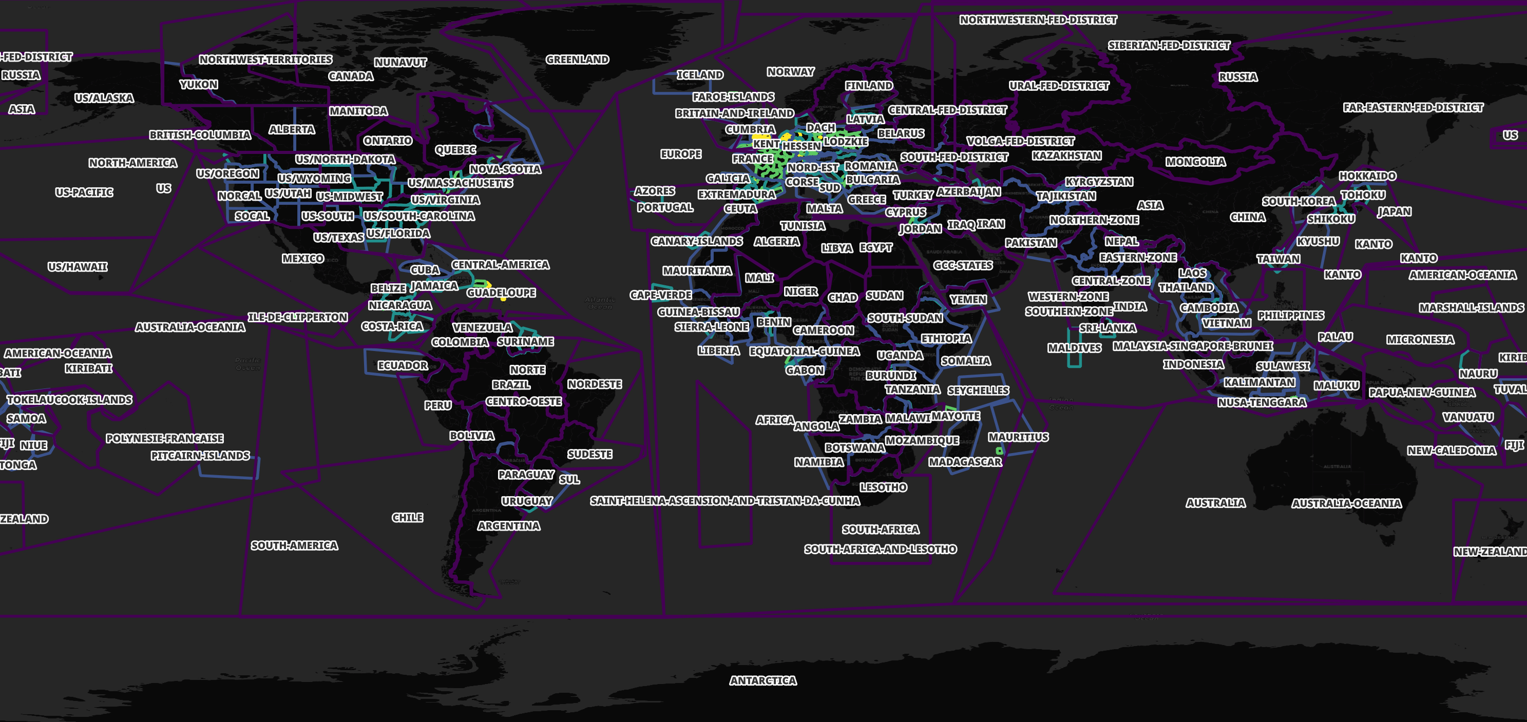
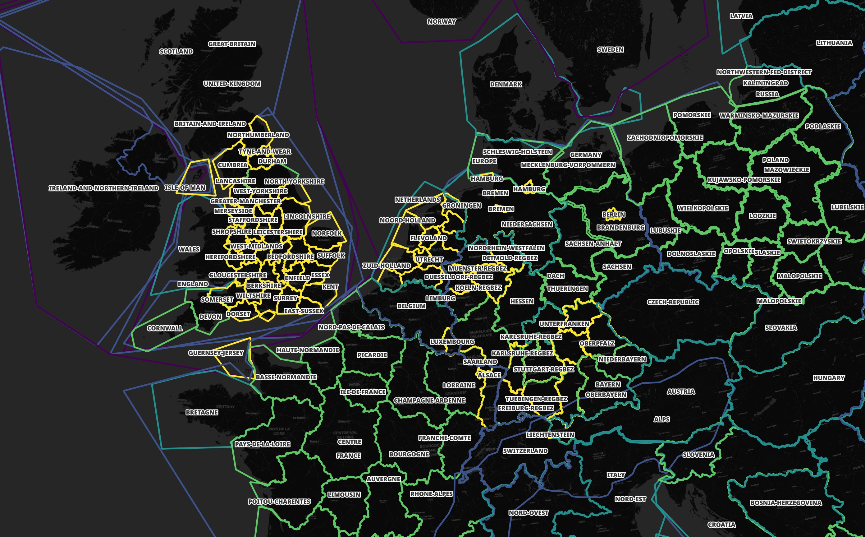
Some areas have more than one file covering their geometry. This allows for downloading smaller files if you're only interested in a certain location or a larger file if you want to explore a larger area. Western Europe is heavily partitioned as shown below.
Below are the Americas, Africa and Europe with their overlapping partitions.
Land Cover Parquet Files
Overture's 84 land cover Parquet files for September are 695 MB - 1.7 GB each. There isn't an obvious file number-to-file size relationship. Below are the ten largest and smallest files.
  Size | File #
---------------
1.7 GB | 42
1.7 GB | 45
1.6 GB | 41
1.4 GB | 34
1.4 GB | 05
1.4 GB | 78
1.4 GB | 00
1.3 GB | 46
1.3 GB | 66
...
781 MB | 49
776 Mb | 29
773 Mb | 17
766 Mb | 76
753 Mb | 68
739 Mb | 67
737 Mb | 70
717 Mb | 51
700 Mb | 48
695 Mb | 75
I'll build bounding boxes for each file and render them in QGIS.
$ ~/duckdb ~/working.duckdb
COPY (
    SELECT   SPLIT_PART(filename, '-', 2) AS pq_num,
             {min_x: MIN(bbox.xmin),
              min_y: MIN(bbox.ymin),
              max_x: MAX(bbox.xmax),
              max_y: MAX(bbox.ymax)}::BOX_2D::GEOMETRY AS geom,
             ST_AREA(geom) AS area
    FROM     READ_PARQUET('/home/mark/land_cover/*.parquet',
                          filename=true)
    GROUP BY filename
) TO 'land_cover_bboxes.gpkg'
  WITH (FORMAT GDAL,
        DRIVER 'GPKG',
        LAYER_CREATION_OPTIONS 'WRITE_BBOX=YES');
The brightness of the box represents the file number. This shows the data is spatially sorted.
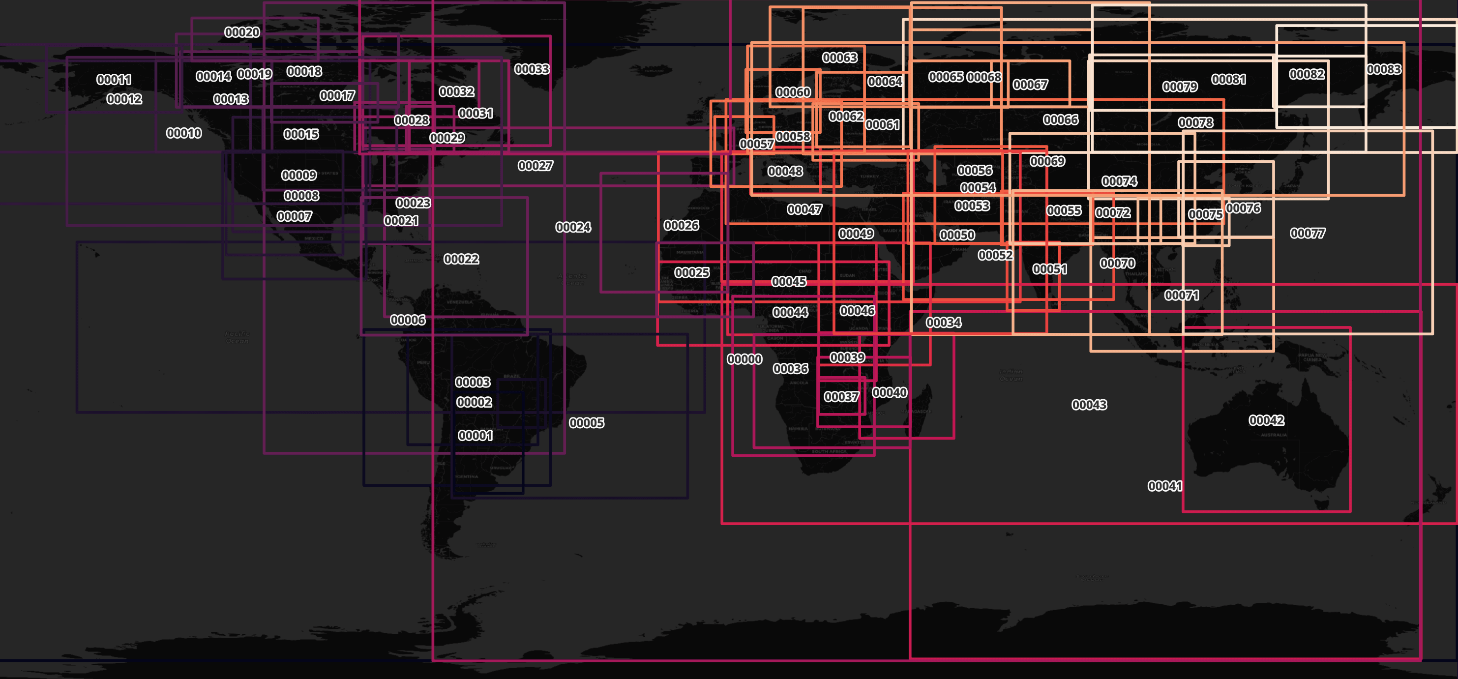
Despite the sorting, the boxes can overlap. Below I've identified five boxes that cover a point in Australia.
SELECT   pq_num
FROM     ST_READ('land_cover_bboxes.gpkg')
WHERE    ST_CONTAINS(geom, ST_POINT(131.95,-22.6))
ORDER BY area;
┌─────────┐
│ pq_num  │
│ varchar │
├─────────┤
│ 00042   │
│ 00043   │
│ 00041   │
│ 00034   │
│ 00000   │
└─────────┘
Most of the geometry is under 1 MB in Well-known Text (WKT) format. Below are the number of records for each Parquet file by their lowest file size in MB bin.
CREATE OR REPLACE TABLE size_bins AS
    SELECT   SPLIT_PART(filename, '-', 2)                AS pq_num,
             ROUND(LEN(geometry::TEXT) / 1024 ** 2)::INT AS MB,
             COUNT(*)                                    AS num_recs
    FROM     READ_PARQUET('/home/mark/land_cover/*.parquet',
                          filename=true)
    GROUP BY 1, 2;

PIVOT    size_bins
ON       MB
USING    SUM(num_recs)
GROUP BY pq_num
ORDER BY "2" DESC,
         "1" DESC;
┌─────────┬─────────┬────────┬────────┐
│ pq_num  │    0    │   1    │   2    │
│ varchar │ int128  │ int128 │ int128 │
├─────────┼─────────┼────────┼────────┤
│ 00025   │ 1363079 │    457 │      7 │
│ 00038   │ 1387537 │    369 │      2 │
│ 00046   │ 1420659 │    398 │      1 │
│ 00066   │ 1427622 │     63 │      1 │
│ 00015   │ 1435221 │      7 │      1 │
│ 00045   │ 1398188 │    744 │        │
│ 00005   │ 1400647 │    543 │        │
│ 00041   │ 1395295 │    505 │        │
│ 00006   │ 1409992 │    482 │        │
│ 00042   │ 1398825 │    475 │        │
│ 00026   │ 1406848 │    364 │        │
│ 00002   │ 1414848 │    361 │        │
│ 00044   │ 1403923 │    358 │        │
│ 00022   │ 1370895 │    341 │        │
│ 00043   │ 1409399 │    333 │        │
│ 00040   │ 1396779 │    331 │        │
│ 00036   │ 1406182 │    290 │        │
│ 00035   │ 1395251 │    287 │        │
│ 00034   │ 1406844 │    283 │        │
│ 00008   │ 1406404 │    278 │        │
│   ·     │    ·    │      · │   ·    │
│   ·     │    ·    │      · │   ·    │
│   ·     │    ·    │      · │   ·    │
│ 00082   │ 1378567 │     18 │        │
│ 00083   │ 1382615 │     16 │        │
│ 00013   │ 1414228 │     13 │        │
│ 00064   │ 1411842 │     10 │        │
│ 00079   │ 1382791 │      8 │        │
│ 00060   │ 1391646 │      4 │        │
│ 00059   │ 1403766 │      3 │        │
│ 00061   │ 1395981 │      3 │        │
│ 00069   │ 1409036 │      3 │        │
│ 00012   │ 1414931 │      1 │        │
│ 00081   │ 1434378 │      1 │        │
│ 00068   │ 1397729 │      1 │        │
│ 00020   │ 1380860 │      1 │        │
│ 00014   │ 1366440 │      1 │        │
│ 00011   │ 1404422 │        │        │
│ 00067   │ 1408138 │        │        │
│ 00062   │ 1396633 │        │        │
│ 00063   │ 1370287 │        │        │
│ 00065   │ 1378926 │        │        │
│ 00080   │ 1417148 │        │        │
├─────────┴─────────┴────────┴────────┤
│ 84 rows (40 shown)        4 columns │
└─────────────────────────────────────┘
GeoFabrik & Overture Partition Mapping
I'll build Parquet files containing Overture's ID for each record joined to GeoFabrik's partition ID. This will give me the continent and country of each record. There will be a few erroneous outliers notably with Russia as will be discussed later on.
$ cd ~/
$ for FILENAME in /home/mark/land_cover/*part-*.parquet; do
      PQ_NUM=`echo $FILENAME | cut -d- -f2`

      echo "
          CREATE OR REPLACE TABLE geofabrik AS
              SELECT * EXCLUDE(urls),
                     REPLACE(urls::JSON->'\$.pbf', '\"', '') AS url
              FROM ST_READ('/home/mark/geofabrik.geojson');

          CREATE OR REPLACE TABLE land_cover AS
              SELECT   a.id                                    AS id,
                       a.subtype                               AS subtype,
                       ST_AREA(a.geometry)                     AS area,
                       LIST(b.id ORDER BY ST_AREA(b.geom))     AS osm,
                       LIST(b.id ORDER BY ST_AREA(b.geom))[-2] AS country,
                       LIST(b.id ORDER BY ST_AREA(b.geom))[-1] AS continent
              FROM     READ_PARQUET('$FILENAME') a
              JOIN     geofabrik b
                  ON ST_CONTAINS(
                        b.geom,
                        ST_CENTROID({
                            min_x: a.bbox.xmin,
                            min_y: a.bbox.ymin,
                            max_x: a.bbox.xmax,
                            max_y: a.bbox.ymax}::BOX_2D::GEOMETRY))
              GROUP BY 1, 2, 3;

          COPY(
              SELECT *
              FROM land_cover
          ) TO 'land_cover.$PQ_NUM.pq'
              (FORMAT         'PARQUET',
               CODEC          'ZSTD',
               ROW_GROUP_SIZE 15000);" \
          | ~/duckdb ~/working.duckdb

  done
The resulting land_cover.000*.pq files are ~28 MB each. I'll group them into a single 2.3 GB, ZStandard-compressed Parquet file. Note this file doesn't contain any geometry. It'll be used to join against Overture's Parquet files.
$ cd ~
$ ~/duckdb ~/working.duckdb
COPY (
    FROM READ_PARQUET('land_cover.000*.pq')
) TO '/home/mark/land_cover_geofabrik.pq'
  (FORMAT         'PARQUET',
   CODEC          'ZSTD',
   ROW_GROUP_SIZE 15000);
Below is an example record.
$ echo "FROM  READ_PARQUET('land_cover_geofabrik.pq')
        LIMIT 1" \
    | ~/duckdb -json \
    | jq -S .
[
  {
    "area": 1.4562408186469817e-06,
    "continent": "south-america",
    "country": "chile",
    "id": "08bcfa8861843fff0005dd37b0f79843",
    "osm": "[argentina, chile, south-america]",
    "subtype": "grass"
  }
]
Land Cover Breakdown
Below is the amount of area for each land cover classification by continent. I'll discuss the erroneous Russia result further in this post.
$ ~/duckdb ~/working.duckdb
WITH a AS (
    SELECT   continent,
             subtype,
             SUM(area)::INT area
    FROM     READ_PARQUET('land_cover_geofabrik.pq')
    GROUP BY 1, 2
)
PIVOT    a
ON       subtype
USING    SUM(area)
GROUP BY continent;
┌───────────────────┬────────┬────────┬────────┬────────┬──────────┬────────┬────────┬────────┬────────┬─────────┐
│     continent     │ barren │  crop  │ forest │ grass  │ mangrove │  moss  │ shrub  │  snow  │ urban  │ wetland │
│      varchar      │ int128 │ int128 │ int128 │ int128 │  int128  │ int128 │ int128 │ int128 │ int128 │ int128  │
├───────────────────┼────────┼────────┼────────┼────────┼──────────┼────────┼────────┼────────┼────────┼─────────┤
│ europe            │     44 │    523 │    615 │    441 │          │     26 │     15 │     38 │     27 │       9 │
│ asia              │   1530 │   1249 │   4596 │   3108 │        7 │    210 │    105 │     56 │     77 │     195 │
│ russia            │      1 │     25 │    113 │     55 │          │      2 │      1 │      0 │      2 │       8 │
│ north-america     │    471 │    421 │   2122 │   2031 │        1 │    319 │    376 │    988 │     30 │      76 │
│ central-america   │      1 │      3 │     52 │     37 │        1 │        │      3 │        │      1 │       2 │
│ south-america     │    247 │    252 │   1579 │    834 │        2 │      1 │    335 │      9 │      9 │      19 │
│ australia-oceania │     67 │     77 │    325 │    869 │        2 │      0 │    231 │      0 │      2 │       2 │
│ africa            │   2292 │    342 │    957 │   1140 │        3 │        │    993 │      0 │     12 │      21 │
│ antarctica        │      1 │        │        │      0 │          │        │        │   3135 │        │         │
└───────────────────┴────────┴────────┴────────┴────────┴──────────┴────────┴────────┴────────┴────────┴─────────┘
This is the breakdown by country.
WITH a AS (
    SELECT   country,
             subtype,
             SUM(area)::INT area
    FROM     READ_PARQUET('land_cover_geofabrik.pq')
    GROUP BY 1, 2
)
PIVOT    a
ON       subtype
USING    SUM(area)
GROUP BY country
ORDER BY forest DESC
LIMIT    25;
┌───────────────────────────┬────────┬────────┬────────┬────────┬──────────┬────────┬────────┬────────┬────────┬─────────┐
│          country          │ barren │  crop  │ forest │ grass  │ mangrove │  moss  │ shrub  │  snow  │ urban  │ wetland │
│          varchar          │ int128 │ int128 │ int128 │ int128 │  int128  │ int128 │ int128 │ int128 │ int128 │ int128  │
├───────────────────────────┼────────┼────────┼────────┼────────┼──────────┼────────┼────────┼────────┼────────┼─────────┤
│ russia                    │     49 │    197 │   3183 │   1438 │          │    156 │     38 │     33 │      6 │     183 │
│ us                        │    106 │    335 │   1465 │    902 │        0 │     34 │     75 │     36 │     23 │      24 │
│ colombia                  │      1 │      1 │    777 │     44 │        0 │      0 │      2 │      0 │      0 │       1 │
│ canada                    │    294 │     62 │    602 │   1011 │          │    263 │    109 │     92 │      3 │      51 │
│ brazil                    │      4 │    133 │    492 │    327 │        1 │        │    165 │        │      5 │       9 │
│ congo-democratic-republic │      0 │      1 │    469 │     86 │        0 │        │     27 │      0 │      0 │       1 │
│ myanmar                   │      1 │     24 │    392 │     10 │        1 │      0 │      0 │      0 │      0 │       0 │
│ china                     │    680 │    335 │    275 │    255 │        0 │     22 │      2 │     11 │     34 │       2 │
│ australia                 │     64 │     76 │    246 │    831 │        1 │        │    231 │      0 │      2 │       2 │
│ indonesia                 │      2 │      9 │    241 │     11 │        2 │        │      1 │        │      2 │       0 │
│ italy                     │      1 │     17 │    179 │     17 │          │      0 │      2 │      0 │      2 │       0 │
│ europe                    │      2 │     32 │    119 │     67 │          │      2 │      1 │      0 │      2 │       8 │
│ india                     │     36 │    370 │    111 │     35 │        0 │      1 │     18 │      3 │      8 │       1 │
│ australia-oceania         │      0 │      0 │     97 │      3 │        2 │        │      0 │      0 │      0 │       1 │
│ japan                     │      1 │      7 │     66 │      1 │        0 │      0 │      0 │      0 │      6 │       0 │
│ peru                      │     17 │      2 │     65 │     67 │        0 │      0 │      8 │      0 │      1 │       0 │
│ guinea                    │      0 │      0 │     62 │     12 │        0 │        │      8 │        │      0 │       0 │
│ sweden                    │      1 │      5 │     56 │     72 │          │      3 │      0 │      0 │      1 │       1 │
│ mexico                    │     23 │     24 │     55 │     39 │        1 │        │    192 │      0 │      3 │       1 │
│ turkey                    │      7 │     40 │     53 │     35 │          │      0 │      1 │      0 │      2 │       0 │
│ tanzania                  │      1 │     32 │     52 │     28 │        0 │        │     39 │      0 │      0 │       1 │
│ chile                     │    109 │      4 │     50 │     46 │          │      1 │      5 │      8 │      1 │       0 │
│ finland                   │      0 │      4 │     48 │      8 │          │      1 │      0 │      0 │      0 │       2 │
│ bolivia                   │     15 │      6 │     47 │     33 │          │        │     10 │      0 │      0 │       1 │
│ venezuela                 │      1 │      1 │     45 │     65 │        0 │        │      8 │      0 │      0 │       1 │
├───────────────────────────┴────────┴────────┴────────┴────────┴──────────┴────────┴────────┴────────┴────────┴─────────┤
│ 25 rows                                                                                                     11 columns │
└────────────────────────────────────────────────────────────────────────────────────────────────────────────────────────┘
There are odd records for Russia that hit GeoFabrik's geometry for neighbouring countries like the US, Poland, Lithuania, etc... If this blog proves popular, I'll look to see if the geometry could be adjusted to correct for these sorts of issues.
.maxrows 10

SELECT   osm,
         COUNT(*)
FROM     READ_PARQUET('land_cover_geofabrik.pq')
WHERE    osm::TEXT LIKE '%russia%'
GROUP BY 1
ORDER BY 2 DESC;
┌─────────────────────────────────────────────────────────────────────────────────────────────────────────────┬──────────────┐
│                                                     osm                                                     │ count_star() │
│                                                  varchar[]                                                  │    int64     │
├─────────────────────────────────────────────────────────────────────────────────────────────────────────────┼──────────────┤
│ [far-eastern-fed-district, russia, asia]                                                                    │      5341951 │
│ [siberian-fed-district, russia, asia]                                                                       │      3820049 │
│ [ural-fed-district, russia, asia]                                                                           │      3516632 │
│ [northwestern-fed-district, russia, asia]                                                                   │       985794 │
│ [volga-fed-district, russia, asia]                                                                          │       772708 │
│                 ·                                                                                           │            · │
│                 ·                                                                                           │            · │
│                 ·                                                                                           │            · │
│ [kaliningrad, podlaskie, warminsko-mazurskie, poland, northwestern-fed-district, europe, russia]            │            3 │
│ [georgia, north-caucasus-fed-district, south-fed-district, europe, russia, asia]                            │            2 │
│ [kaliningrad, podlaskie, warminsko-mazurskie, lithuania, poland, northwestern-fed-district, europe, russia] │            1 │
│ [azerbaijan, north-caucasus-fed-district, europe, russia, asia]                                             │            1 │
│ [podlaskie, warminsko-mazurskie, lithuania, poland, northwestern-fed-district, europe, russia]              │            1 │
├─────────────────────────────────────────────────────────────────────────────────────────────────────────────┴──────────────┤
│ 78 rows (10 shown)                                                                                               2 columns │
└────────────────────────────────────────────────────────────────────────────────────────────────────────────────────────────┘
SELECT   country,
         continent,
         COUNT(*)
FROM     READ_PARQUET('land_cover_geofabrik.pq')
WHERE    osm::TEXT LIKE '%russia%'
GROUP BY 1, 2
ORDER BY 3 DESC;
┌───────────────┬───────────┬──────────────┐
│    country    │ continent │ count_star() │
│    varchar    │  varchar  │    int64     │
├───────────────┼───────────┼──────────────┤
│ russia        │ asia      │     15778733 │
│ europe        │ russia    │      1428737 │
│ north-america │ asia      │       153588 │
└───────────────┴───────────┴──────────────┘
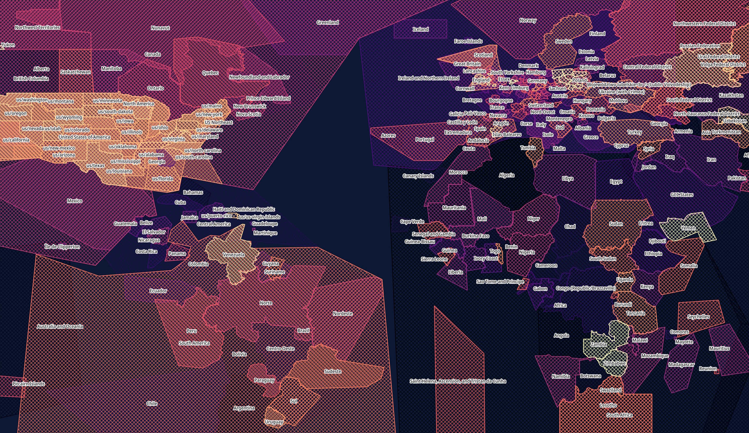
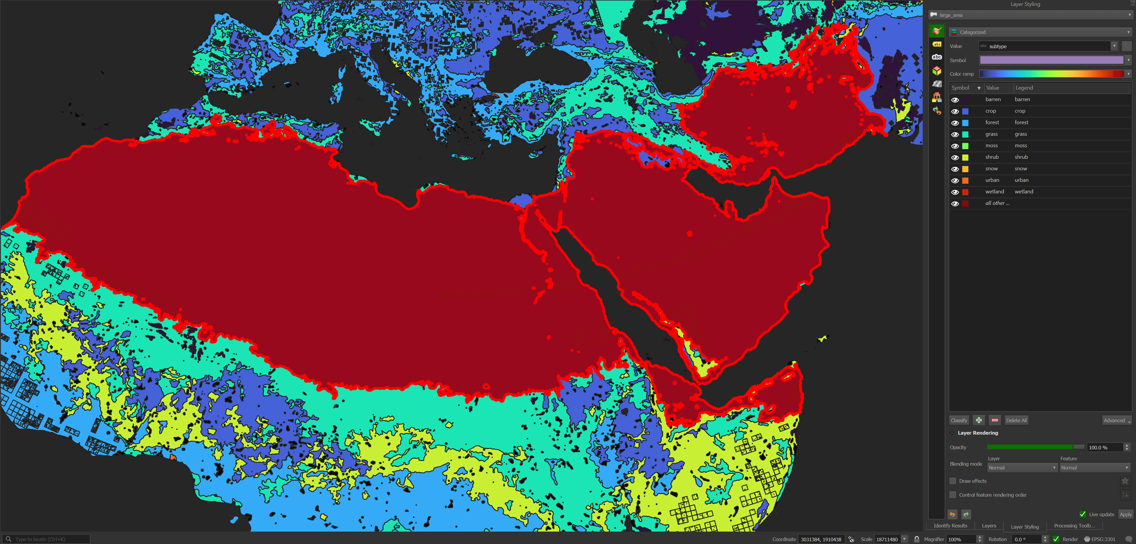
Very Large Polygons
The centroid of each piece of geometry is used to determine the point that will be used to map to GeoFabrik's partitions. In some cases, a polygon or multi-polygon can cover more than a single country and in the extreme case below, a single record's polygons can cover almost the entirety of North Western Africa to Central Asia. This is another edge case I need to look at.
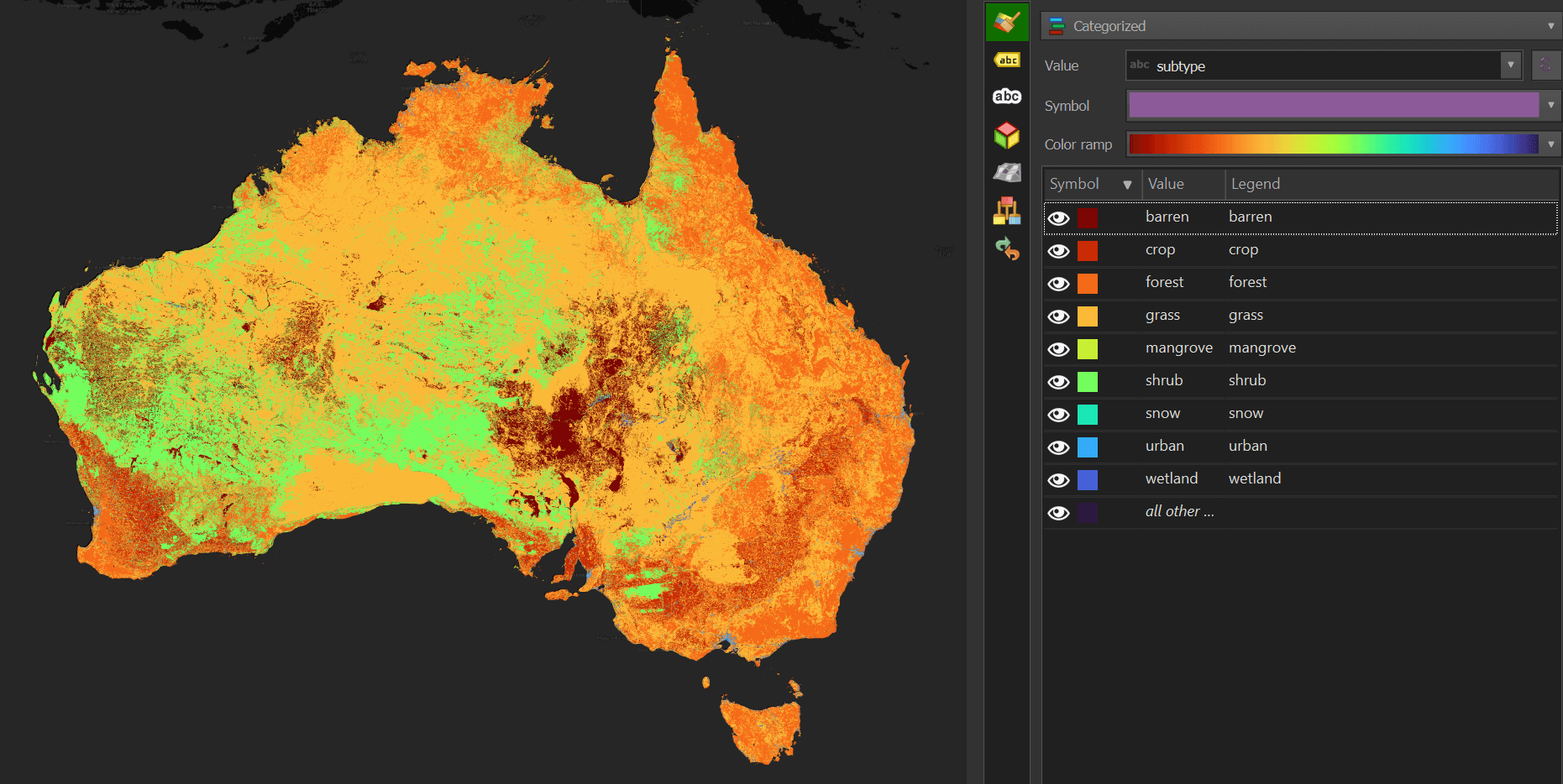
Extract Australian Land Cover Data
The following will produce a 3.6 GB, 2,536,022-record Parquet file for Australia. Some geometry in the dataset covers much of Australia and if rendered after smaller geometry in the same area, could end up covering it. I've sorted the geometry so the largest polygons appear first. This means QGIS will render them before any smaller geometry which overlaps with them.
$ ~/duckdb ~/working.duckdb
COPY (
    SELECT   b.subtype subtype,
             b.geometry as geom
    FROM     READ_PARQUET('/home/mark/land_cover_geofabrik.pq') a
    JOIN     READ_PARQUET('/home/mark/land_cover/*.parquet') b ON a.id = b.id
    WHERE    a.country = 'australia'
    ORDER BY a.area DESC
) TO 'australia.pq'
     (FORMAT         'PARQUET',
      CODEC          'ZSTD',
      ROW_GROUP_SIZE 15000);
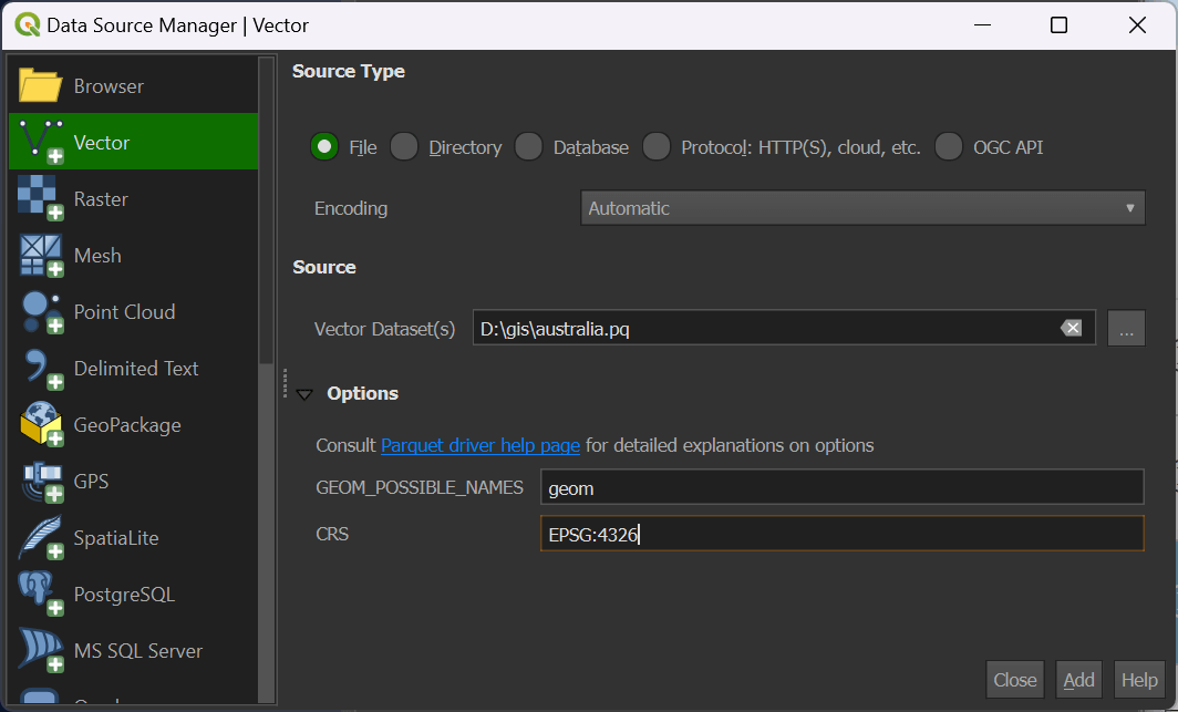
Unlike GeoPackage (GPKG) files, Parquet files can't be opened by dropping them onto QGIS.
In a new QGIS workspace, click on the Layer Menu -> Add Layer -> Add Vector Layer.
Select the location where you saved australia.pq.
Set the geometry field name to "geom" and the projection to "EPSG:4326".
Below is a rendering of Australia's land cover dataset in Overture's September release broken down by type of cover.