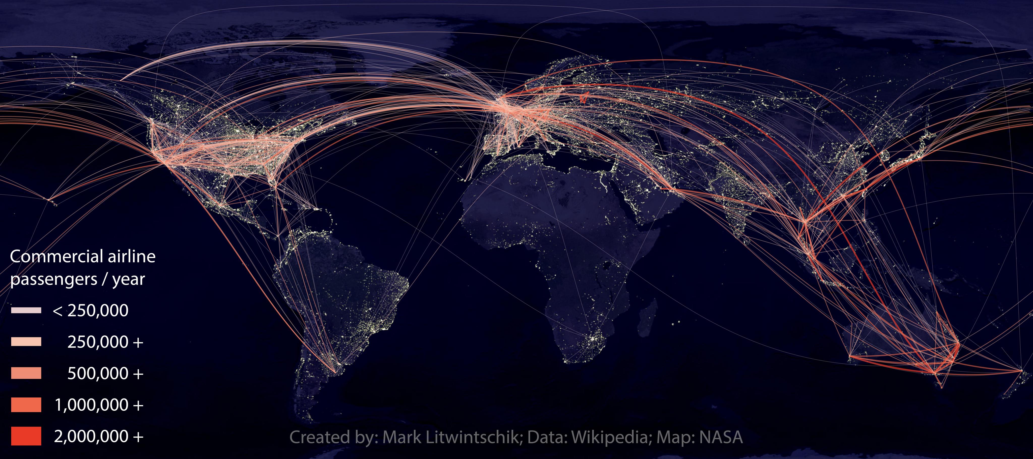
This map represents some of the most popular commercial airline routes. Each route is coloured and given a line width to represent how many people in the latest year reported flew between two given airports.
The Data Collection Process
When I started the data collection process for this map I knew not every airport page on Wikipedia reported how many passengers flew to and from the destinations they connect with. But I suspected I could fill in the blanks if the other destinations reported what passenger counts they were seeing.
Neither of Moscow's two big airports, Sheremetyevo and Domodedovo, report how many passengers travel to and from their top destinations on their Wikipedia pages. But Bangkok's Suvarnabhumi Airport Wikipedia page reports that 266,889 and 316,055 passengers flew to and from Sheremetyevo and Domodedovo respectively in 2013. Novosibirsk's Tolmachevo did report 215,408 passengers coming and going in 2013 from Bangkok's Suvarnabhumi which lines up closely with 212,715 reported on Suvarnabhumi's Wikipedia page.
Prague Airport and Charles de Gaulle Airport reported 637,566 and 790,922 passengers respectively flying between their airports and Sheremetyevo. But others, like Kiev's Boryspil grouped passenger counts by major city by combining the numbers for Domodedovo and Sheremetyevo.
The routes for Sheremetyevo & Sharm el-Sheikh, Sheremetyevo & Krasnodar, Sheremetyevo & Kaliningrad had no reported passenger numbers at all. A large part of passenger traffic in China, India, Brazil and South Africa isn't broken down by destination/arrival airport.
Of the 28,731 wikipedia articles I found with a title that has 'Airport' in it I extracted 5,958 airport entities and 343^ of those airports had passenger counts broken down by destinations they connect with. Most of the said pages had at least the top 10 connecting airports with corresponding passenger counts for the year, many had the top 20 and a few stars (mostly in Western Europe and South East Asia) had over 50.
^ This number is probably higher but 343 was all my parser could sort out.
Setting up an Environment
I installed a few tools on my Ubuntu 14.04 machine to collect the data and render it out.
$ sudo apt update
$ sudo apt install \
    python-mpltoolkits.basemap \
    pandoc \
    libxml2-dev \
    libxslt1-dev \
    redis-server
$ sudo pip install docopt
I almost exclusively work in a virtual environment, and in the collection phase of this project I did but the BaseMap package used by Matplotlib wasn't playing nice when I tried to install it via pip so I chose to go with the Ubuntu distribution.
I moved the map rendering tasks out to plot.py. For all the work I did in app.py I had a virtual environment setup with 11 packages:
$ virtualenv passengers
$ source passengers/bin/activate
$ pip install -r requirements.txt
When switching from the collection process to the rendering process you can exit the virtual environment with the following:
$ deactivate
Download a copy of Wikipedia
If I can avoid making tens of thousands of network requests, even via a queue, to a remote server then I'll do my best to do so. For this task I decided to download ~11GB of Wikipedia's English-language articles. There is a single file you can download or you can do it in chunks:
$ wget -c https://dumps.wikimedia.org/enwiki/20150702/enwiki-20150702-pages-articles1.xml-p000000010p000010000.bz2
$ wget -c https://dumps.wikimedia.org/enwiki/20150702/enwiki-20150702-pages-articles2.xml-p000010002p000025001.bz2
$ wget -c https://dumps.wikimedia.org/enwiki/20150702/enwiki-20150702-pages-articles3.xml-p000025001p000055000.bz2
$ wget -c https://dumps.wikimedia.org/enwiki/20150702/enwiki-20150702-pages-articles4.xml-p000055002p000104998.bz2
$ wget -c https://dumps.wikimedia.org/enwiki/20150702/enwiki-20150702-pages-articles5.xml-p000105002p000184999.bz2
$ wget -c https://dumps.wikimedia.org/enwiki/20150702/enwiki-20150702-pages-articles6.xml-p000185003p000305000.bz2
$ wget -c https://dumps.wikimedia.org/enwiki/20150702/enwiki-20150702-pages-articles7.xml-p000305002p000465001.bz2
$ wget -c https://dumps.wikimedia.org/enwiki/20150702/enwiki-20150702-pages-articles8.xml-p000465001p000665001.bz2
$ wget -c https://dumps.wikimedia.org/enwiki/20150702/enwiki-20150702-pages-articles9.xml-p000665001p000925001.bz2
$ wget -c https://dumps.wikimedia.org/enwiki/20150702/enwiki-20150702-pages-articles10.xml-p000925001p001325001.bz2
$ wget -c https://dumps.wikimedia.org/enwiki/20150702/enwiki-20150702-pages-articles11.xml-p001325001p001825001.bz2
$ wget -c https://dumps.wikimedia.org/enwiki/20150702/enwiki-20150702-pages-articles12.xml-p001825001p002425000.bz2
$ wget -c https://dumps.wikimedia.org/enwiki/20150702/enwiki-20150702-pages-articles13.xml-p002425002p003125001.bz2
$ wget -c https://dumps.wikimedia.org/enwiki/20150702/enwiki-20150702-pages-articles14.xml-p003125001p003925001.bz2
$ wget -c https://dumps.wikimedia.org/enwiki/20150702/enwiki-20150702-pages-articles15.xml-p003925001p004824998.bz2
$ wget -c https://dumps.wikimedia.org/enwiki/20150702/enwiki-20150702-pages-articles16.xml-p004825005p006025001.bz2
$ wget -c https://dumps.wikimedia.org/enwiki/20150702/enwiki-20150702-pages-articles17.xml-p006025001p007524997.bz2
$ wget -c https://dumps.wikimedia.org/enwiki/20150702/enwiki-20150702-pages-articles18.xml-p007525004p009225000.bz2
$ wget -c https://dumps.wikimedia.org/enwiki/20150702/enwiki-20150702-pages-articles19.xml-p009225002p011124997.bz2
$ wget -c https://dumps.wikimedia.org/enwiki/20150702/enwiki-20150702-pages-articles20.xml-p011125004p013324998.bz2
$ wget -c https://dumps.wikimedia.org/enwiki/20150702/enwiki-20150702-pages-articles21.xml-p013325003p015724999.bz2
$ wget -c https://dumps.wikimedia.org/enwiki/20150702/enwiki-20150702-pages-articles22.xml-p015725013p018225000.bz2
$ wget -c https://dumps.wikimedia.org/enwiki/20150702/enwiki-20150702-pages-articles23.xml-p018225004p020925000.bz2
$ wget -c https://dumps.wikimedia.org/enwiki/20150702/enwiki-20150702-pages-articles24.xml-p020925002p023725001.bz2
$ wget -c https://dumps.wikimedia.org/enwiki/20150702/enwiki-20150702-pages-articles25.xml-p023725001p026624997.bz2
$ wget -c https://dumps.wikimedia.org/enwiki/20150702/enwiki-20150702-pages-articles26.xml-p026625004p029624976.bz2
$ wget -c https://dumps.wikimedia.org/enwiki/20150702/enwiki-20150702-pages-articles27.xml-p029625017p047137381.bz2
Make the Data Smaller
As a single step I wanted to extract all the article titles and bodies from the XML files where 'Airport' appeared in the title. This process took over an hour on my machine and the result was that I didn't need to repeat this step if and when future steps failed.
$ python app.py get_wikipedia_content title_article_extract.json
This process turned ~11GB of compressed articles into a 68MB uncompressed JSON file. I was happy to see Python's standard library did almost everything I needed to achieve this:
import bz2
import codecs
from glob import glob

from lxml import etree


def get_parser(filename):
    ns_token        = '{http://www.mediawiki.org/xml/export-0.10/}ns'
    title_token     = '{http://www.mediawiki.org/xml/export-0.10/}title'
    revision_token  = '{http://www.mediawiki.org/xml/export-0.10/}revision'
    text_token      = '{http://www.mediawiki.org/xml/export-0.10/}text'

    with bz2.BZ2File(filename, 'r+b') as bz2_file:
        for event, element in etree.iterparse(bz2_file, events=('end',)):
            if element.tag.endswith('page'):
                namespace_tag = element.find(ns_token)

                if namespace_tag.text == '0':
                    title_tag = element.find(title_token)
                    text_tag = element.find(revision_token).find(text_token)
                    yield title_tag.text, text_tag.text

                element.clear()


def pluck_wikipedia_titles_text(pattern='enwiki-*-pages-articles*.xml-*.bz2',
                               out_file='title_article_extract.json'):
    with codecs.open(out_file, 'a+b', 'utf8') as out_file:
        for bz2_filename in sorted(glob(pattern),
                                   key=lambda a: int(
                                        a.split('articles')[1].split('.')[0]),
                                   reverse=True):
            print bz2_filename
            parser = get_parser(bz2_filename)

            for title, text in parser:
                if 'airport' in title.lower():
                    out_file.write(json.dumps([title, text],
                                              ensure_ascii=False))
                    out_file.write('\n')
The files are processes in descending order as the largest files came last and I wanted to know about any memory and recursion issues early on.
Converting Wikipedia's Markdown into HTML
When I first started exploring the idea of making this map I downloaded the HTML of a few airport pages from Wikipedia and used BeautifulSoup to parse the airport characteristics and passenger counts out. The process was easy to write and worked well on the few examples I presented it with. But the article data I've downloaded from Wikipedia is in their own Markdown flavour and needs to be converted into HTML.
I experimented with creole and pandoc for doing the conversion. Both had mixed results. Not all airport pages are written in the same fashion so even though the data is there it can be structured very differently on two different pages. Infoboxes and tables did not render into HTML properly at all. In some cases every cell in a table would show up as its own row.
In order to keep this task in the time box I assigned to it I decided to try three ways of extracting the data I wanted: try creole, if I couldn't parse out the data I needed I then tried pandoc. If pandoc didn't work out I manually connected out to Wikipedia's site and scraped the HTML from them. I didn't want to hammer Wikipedia's servers with requests so I limited the calls to 3 every 10 seconds and cached the results in Redis.
import ratelim
import redis
import requests


@ratelim.greedy(3, 10) # 3 calls / 10 seconds
def get_wikipedia_page_from_internet(url_suffix):
    url = 'https://en.wikipedia.org%s' % url_suffix
    resp = requests.get(url)
    assert resp.status_code == 200, (resp, url)
    return resp.content


def get_wikipedia_page(url_suffix):
    redis_con = redis.StrictRedis()
    redis_key = 'wikipedia_%s' % sha1(url_suffix).hexdigest()[:6]
    resp = redis_con.get(redis_key)

    if resp is not None:
        return resp

    html = get_wikipedia_page_from_internet(url_suffix)
    redis_con.set(redis_key, html)

    return html
If there was a connection issue or one of the page links given was to a page that didn't exist the script would just carry on to the next page:
try:
    html = get_wikipedia_page(url_key)
except (AssertionError, requests.exceptions.ConnectionError):
    pass # Some pages link to 404s, just move on...
else:
    soup = BeautifulSoup(html, "html5lib")
I found some of the HTML would render so poorly that it would cause BeautifulSoup to hit recursion depth limits set in CPython. When this happened I just moved on to the next page knowing that I could handle some missing data and good is not the enemy of perfect.
try:
    soup = BeautifulSoup(html, "html5lib")
    passenger_numbers = pluck_passenger_numbers(soup)
except RuntimeError as exc:
    if 'maximum recursion depth exceeded' in exc.message:
        passenger_numbers = {}
    else:
        raise exc
The command to pluck out the airport properties and connections details is as follows:
$ python app.py pluck_airport_meta_data \
                title_article_extract.json \
                stats.json
Picking a Design for the Map
I didn't want this data to render as a bar chart but plotting lines on a map of the Earth which is coloured in bright blue and green would just leave me with an image that felt noisy.
Luckily, I came across a blog post by James Cheshire, a lecturer at the UCL Department of Geography, where he critiques maps put together by Michael Markieta. Michael had plotted flight routes from four airports in London to destinations they connected to around the world. The map of Earth used was the Night lights map put together by NASA.
I had struggled to find a colour scheme that separated the routes visually and the pink to red scheme he used seem to work well. I found a scheme similar at Color Brewer 2.0. In addition to the colour, I varied the transparency and line width based on how many passengers had used a route in a given year.
display_params = (
    # color   alpha  width threshold
    ('#e5cccf', 0.3, 0.2, 0),
    ('#f7c4b1', 0.4, 0.3, 250000),
    ('#ed8d75', 0.5, 0.4, 500000),
    ('#ef684b', 0.6, 0.6, 1000000),
    ('#e93a27', 0.7, 0.8, 2000000),
)

for iata_pair, passenger_count in pairs.iteritems():
    colour, alpha, linewidth, _ = display_params[0]

    for _colour, _alpha, _linewidth, _threshold in display_params:
        if _threshold > passenger_count:
            break

        colour, alpha, linewidth = _colour, _alpha, _linewidth
Rendering the Map
Using the Basemap package to render the map was reasonably straight forward. The only issue I ran up against was routes crossing the Pacific Ocean would stop at the edge of the image, draw a straight line across to the other side of the image and then continue on to their destination. It's a documented problem in the documentation for the drawgreatcircle method.
Phil Elson, a core developer on matplotlib, came up with a solution that fixed this issue.
line, = m.drawgreatcircle(long1, lat1, long2, lat2,
                                  linewidth=linewidth,
                                  color=colour,
                                  alpha=alpha,
                                  solid_capstyle='round')

p = line.get_path()

# Find the index which crosses the dateline (the delta is large)
cut_point = np.where(np.abs(np.diff(p.vertices[:, 0])) > 200)[0]

if cut_point:
    cut_point = cut_point[0]

    # Create new vertices with a nan in between and set
    # those as the path's vertices
    new_verts = np.concatenate([p.vertices[:cut_point, :],
                                [[np.nan, np.nan]],
                                p.vertices[cut_point+1:, :]])
    p.codes = None
    p.vertices = new_verts
The commands to render a PNG and an SVG map are as follows:
# Exit the virtual environment in order to use the system-wide
# Basemap package:
$ deactivate

$ python plot.py render stats.json out.png
$ python plot.py render stats.json out.svg
See what you can do with the data
I've made the airport IATA code pairs and passenger volumes available as a CSV.
The routes plotted on the night lights image from from NASA are available as an SVG file. This should allow someone with good Illustrator skills to further stylise the map.
The Python code used to pull the data together and plot it on the map is available on GitHub.